Understanding the S-Domain

Introduction

Because I often create and solve s-domain equations in my articles to analyze circuits, I thought it well to present here a brief explanation of the s-domain.

Mathematical Difficulties

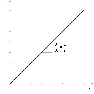
Circuit analysis would be a simple case of adding series and parallel resistors and doing related calculations as in DC analysis if not for the addition of the energy storage components: the inductor and capacitor. In figure 1 below the inductor charges current at a rate proportional to the voltage drop across it. Likewise in figure 2 below the capacitor charges voltage at a rate proportional to its input current.

Figure 1: Current increases through inductor as it charges.		Figure 2: Voltage increases across capacitor as it charges

Unfortunately these component behaviors are mathematically modeled by the calculus operation of differentiation, or integration if the equations are reversed with respect to voltage and current. Differentiation represented in figures 1 and 2 above is simply the instantaneous slope of the input function.

(1)

v = L

(2)

i = C

Direct circuit analysis with calculus level math then requires putting these operations together to solve them in a form called the differential equation:

(3)

D(t) = a₀f(t) + a₁

d f(t)

+ a₂

d² f(t)

dt²

+ a₃

d³ f(t)

dt³

+ … + a_n

dⁿ f(t)

dtⁿ

where

dⁿ f(t)

dtⁿ

represents the function f(t) differentiated n times.

Arbitrary differential equations are only sensible if they represent functions that have the same form only altered in scale when differentiated or integrated. Because exponential and sinusoid functions always follow this rule, it is usually assumed that the solution to such a differential equation is a function of this sort. If it is further assumed that sinusoids are derived from an exponential with an imaginary power (i.e. Euler's Law: e^jx = cos(x) + jsin(x)), additional generalization of the solution function will result.

(4)

f(t) = e^st

^a where s = σ + jω

Each level of differentiation multiplies the solution equation by s.

(5)

d e^st

= se^st

If this generalized solution equation is substituted for f(t) a considerable simplification can be affected.

(6)

D(t) = a₀e^st + a₁

d e^st

dt¹

+²a₂

d² e^st

dt²

+³a₃

d³ e^st

dt³

+ … +ⁿa_n

dⁿ e^st

dtⁿ

Differentiating each term multiplies it by a power of s of the same degree as the derivative.

(7)	D(t) = a₀e^st + a₁se^st + a₂s²e^st + a₃s³e^st + … + a_nsⁿe^st

Now dividing the entire equation by the generalized solution leaves a simple polynomial in the s-domain that is much easier manipulated and solved.

(8)	D(s) = a₀ + a₁s + a₂s² + a₃s³ + … + a_nsⁿ

This transformation of a differential equation to an algebraic one in a complex variable is known generally as the Laplace Transformation. Where F(s) is the Laplace transform of f(t) the following integral defines this transformation.

(9)

F(s) =

∫

∞

0

e^-stf(t)

Simplified AC Analysis

Performing the same reductions steps on the defining differential equations 1 and 2 for the inductor and capacitor gives s-domain terms for their impedance that can be used to solve circuit equations with simple algebra rather than the calculus on which they are based. Because the Laplace transform is linear, the transforms of the individual components can be added together.

(10)

Z_L = sL

(11)

Z_C =

These simple s-domain representations of otherwise complicated calculus can be used in serial, parallel, and other DC equations and then solved with regular algebra.

(12)	Z_SERIES = Z₁ + Z₂		(13)	Z_PARALLEL =	Z₁Z₂ Z₁ + Z₂
(14)	Y_PARALLEL = Y₁ + Y₂		(15)	Y_SERIES =	Y₁Y₂ Y₁ + Y₂

The simple reduced s-domain equation of equation 8 above contains only zeros when factored and is likely only to occur in a series RL impedance or a parallel RC conductance. In other cases reduction of an s-domain equation will yield an equation with zeros in the numerator and poles in the denominator. Zeros are zero at their characteristic s-value and poles represent infinity at theirs.

(16)

H(s) =

a₀ + a₁s + a₂s² + a₃s³ + … + a_ms^m

b₀ + b₁s + b₂s² + b₃s³ + … + b_nsⁿ

(17)

H(s) =

(s - z₁)(s - z₂)(s - z₃) … (s - z_m)

(s - p₁)(s - p₂)(s - p₃) … (s - p_n)

What does s actually represent?

The Math

S is a two-dimensional number, a vector, in a form commonly used in mathematics called a complex number. Because complex numbers have unique properties beyond a mere vector some prefer to call them phasors instead. In the form s = σ + jω, σ is a vector component oriented at zero degrees and jω a vector vector component oriented at ninety degrees. j is just a 90º angle marker allowing the vector to be easily represented as an addition or a subtraction in which case -j would represent 270º.

Complex numbers have the following properties:

The 90º vector j is defined as:

(18)

j =

-1

therefore

(19)	j × j = -1

and

(20)

= -j

They have a magnitude:

(21)

|(a + jb)|²=

a² + b²

and a phase angle:

(22)

Phase(a + jb) = arctan

Note: This is a four quadrant arctangent. A calculator arctangent will only be valid for complex numbers with a positive real part. If the real part is negative, the arctangent will have to be adjusted by adding 180º.

(23)

Phase(a + jb) = 180º + arctan

They also have complex conjugate:

(24)	(a + jb)* = a - jb

They can be represented in rectangular form

(25)

a + jb

or polar form:

(26)	\|a + jb\| ∠ Phase(a + jb)

Addition and subtraction are done individually in the real and imaginary parts:

(27)	(a + jb) + (c + jd) = (a + c) + j(b + d)
(28)	(a + jb) - (c + jd) = (a - c) + j(b - d)

In multiplication and division, the real and imaginary parts interact to produce the following results:

(29)	(a + jb) × (c + jd) = (ac-bd) + j(ad+bc) = (\|a + jb\| × \|c + jd\|) ∠ (Phase(a + jb) + Phase(c + jd))

(30)

(a + jb)

(c + jd)

(a + jb) × (c - jd)

(c + jd) × (c - jd)

(ac+bd)²+ j(bc-ad)

c² + d²

|a + jb|

|c + jd|

∠ (Phase(a + jb) - Phase(c + jd))

The Time Domain Significance

Apart from the complex math, an s variable represents a signal in the form the product of an exponential and a sinusoid as the following derivations show.

(31)	f(t) = e^st
(32)	f(t) = e^(σ+jω)t
(33)	f(t) = e^σt(cos(ωt) + jsin(ωt))

Thus σ represents damping and ω a frequency component in natural frequency units of radians/s.

To this point the derivation leaves a paradox: the time-based signal has an imaginary component, something it should not have. In order to resolve the dilemma, try again with the signal divided into normal and complex-conjugate parts.

(34)	f(t) = ½e^st + ½e^s*t
(35)	f(t) = ½e^(σ+jω)t+ ½e^(σ-jω)t
(36)	f(t) = ½e^σt(cos(ωt) + jsin(ωt)) + ½e^σt(cos(ωt) - jsin(ωt))
(37)	f(t) = e^σtcos(ωt)

For this reason, all real signals and systems represent frequencies with positive and negative parts and have poles and zeros in conjugate pairs.

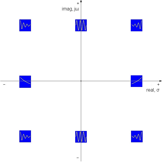
Figure 3 below shows what kind of signals are represented in different locations in the s-domain. Those on the real axis represent only exponential decay and lack a resonant frequency. Those on the imaginary axis represent only a sinusoidal signal without an exponential component. Those left of the imaginary axis but off of the real one are damped sinusoids. Those right of the imaginary axis are all unstable due to exponential increase.

Figure 3: S-domain showing time signal representations.

The Frequency Significance of the S-domain

If jω for a range of frequencies [ω₁ = 2πf₁ … ω_n = 2πf_n] is substituted for s in a full s-equation like equation 16 above, each frequency point will calculate to a concrete s-value representing magnitude and phase the total of which will plot the magnitude or phase frequency response. Equation 16 reduces to the following following equation on the way to yielding concrete numbers. Note that the coefficients now alternate in sign as a result of the way powers of j progress.

(38)

H(ω) =

(a₀- a₂ω² + a₄ω⁴ - …) + j(a₁ω - a₃ω³ + a₅ω⁵ - …)

(b₀ - b₂ω² + b₄ω⁴ - …) + j(b₁ω - b₃ω³ + b₅ω⁵ - …)

Even though s itself is two-dimensional, the plot of an s-equation is three dimensional (or even four dimensional if the complex nature of the results are considered) as if σ and ω defined the base of the plot and the magnitude or phase plots the altitude of a mathematical landscape. Reducing the s-equation with jω slices this three-dimensional plot along the imaginary axis yielding back a two dimensional frequency plot spanning both positive and negative frequencies. Poles and zeros on this landscape do not affect resonance or frequency response as you would expect at this point. You would expect frequency affects to directly correspond their imaginary component jω. Instead frequency effects are correlated to the vector magnitude of their place in the s-domain.

Consider the multiplication of two conjugate poles in a second order lowpass equation.

(39)

H(s) =

(s +²a+jb)(s + a -jb)

s² + 2as + a²+b²

Compare this with the standard equation.

(40)

H(s) =

k
____________

s² +

s + ω²

Solving for the resonance frequency returns the magnitude of the conjugate poles a result arising from the nature of complex math.

(41)	ω² =	a² + b²
(42)	ω²=	a² + b²	=²\|a + jb\|

For completeness at this point, lets solve for Q.

(43)	Q ω	=	1 2a
(44)	Q	=	ω² 2a	=	a² + b² 2a	=	1² 2cos(θ_pole -180º)

Or for simpler calculations Q reduces to:

(45)

Q =

2|cos(θ_pole)|

How convenient! Q is a function of the angle of the pole.

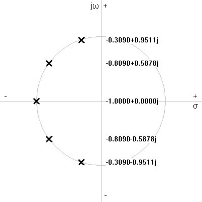
In this light, all the poles in the s-domain pole plot of figure 4 below represent the same frequency as a result of having all the same magnitude. The complex conjugate pairs each correspond to a resonant frequency f₀ and the real pole on the σ axis to a -3dB cutoff frequency f_c.

Figure 4: S-domain plot showing normalized fifth-order lowpass Butterworth response

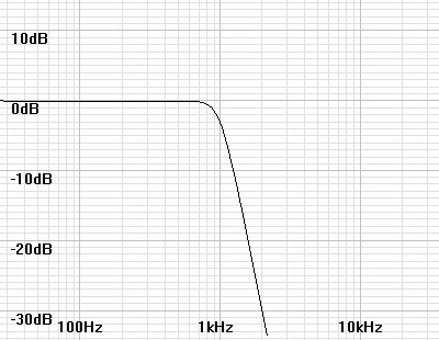
Figure 5: Bode plot shows magnitude response of transfer function represented in pole-zero plot of figure 4 above scaled to 1kHz.

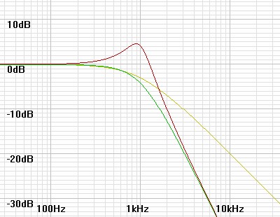
Figure 6: Broken down by pole pairs, the bode plot shows how the nearness of a pole to the jω axis raises Q.

Color	Q	Corresponding normalized pole(s)
yellow	NA	-1 + j0
green	0.618	-0.809 ± j0.5878
red	1.618	-0.309 ± j0.9511

Examples

Examples of the use and manipulation of s-domain equations may be found in the following articles.

Phono Equalization Calculations
Phono Termination Calculations and Calculator
Active Inductor Load
Warp Filter

Last Note

I may return to clarify any points that seem unclear at any point.

Document History
October 26, 2012 Created.
October 27, 2012 Added Q to legend of figure 6 and another link under examples.