 |
| Home │ Audio
Home Page |
Copyright © 2016 by Wayne Stegall
Updated March 21, 2017. See Document History at end for
details.
|
|
Sealed-box Speaker Equalizer
Part 1:
Chebychev design
methods allow the design of speaker equalizer
Introduction
Perhaps you thought Chebychev filters undesirable for audio because of transient overshoot. That is true for electronics. However speaker design regularly uses the Chebychev filter alignment. Indeed, it would be pointless to design a ported speaker with Bessel or Butterworth alignment. Here Chebychev calculations are used to extend the response of sealed box speakers. Sealed box speakers are functionally mechanical second-order filters for woofer and enclosure operation. Therefore adding an appropriate second-order electronic stage will create a fourth-order Chebychev response with a lower cutoff frequency.Calculations
First calculate 4th order Butterworth poles.| (1) |
θpole-i = 90° + |  |
180° × (2i – 1)
2N |
 |
| (2) |
αi + jβi = cos(θpole-i) + jsin(θpole-i) |
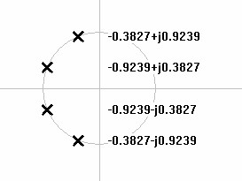
| Figure 1: 4th order lowpass Butterworth pole plot. |
 |
Then one 4th order Chebychev pole is calculated on the unit circle from the speaker Q.
| (3) |
α2'' = | –1
2Qspkr |
| (4) |
β2'' = | 1 – α2'2 |
Then that pole is scaled so that the imaginary part has the same value as the corresponding 2nd Butterworth pole.
| (5) |
α2' + jβ2' = (α2'' + jβ2'') × | α2
α2'' |
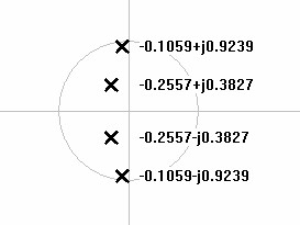
| Figure 2: Typical 4th order lowpass Chebychev pole plot. |
 |
Now the ratio of the real part of the Chebychev pole to the real part of the Butterworth pole gives the Chebychev constant.
| (6) |
kcheby = |
α2'
α2 |
kcheby is all that is necessary to design the filter, however it is desirable to calculate the resulting 4th order design parameters at this time.
| (7) |
A = tan-1(kcheby) |
| (8) |
ε = |
1
sinh(A × n) |
| (9) |
rippledB = 10 × log10(ε2 + 1) |
| (10) |
f3dB = fspkr × | α2'2 + β2'2 |
| (11) |
fripple = f3dB × cosh(A) |
Now using kcheby calculate first Chebychev pole representing the filter.
| (12) |
α1' + jβ1' = kcheb⋅α1 + jβ1 |
Then calculate filter Q and resonant frequency.
| (13) |
Qfilter = |
1
2cosθ |
= |
α1'2 + β1'2
2α1' |
| (14) |
ffilter = |
f3dB
|
Program
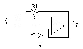
Because this article pertained to an actual application, I decided to present a program rather than just an example. The program of figure 4 calculates the filter, shows its specifications, then prints the SPICE model for it. The resulting SPICE model represents the topology show below in figure 3.and is verified to run on SPICE Opus. I chose C++ for the program rather than C because I wanted to use complex numbers.| Figure
3:
Unity
gain
VCVS
filter
topology
chosen
for
program. |
 |
| Figure
4:
Code
listing
for
filter
program
sbeq.cpp: |
| #include <iostream> #include <complex> #include <stdio.h> #include <math.h> // #include <mathext.h> //include inverse hyperbolic functions. using namespace std; #define ORDER 4 #define sqr(x) ((x)*(x)) int main(int argc, char* argv[]) { int p, ret; double qmin,f,q,f2,f3db,fripple,q2,thetap,pi,kcheby,A,epsilon,dbripple; double fsf, c1c2, c1c2u, r1[2], r2[2]; complex <double> buttp[2], chebp[2]; pi = acos(-1); // calculate first two poles of 4th order Butterworth for(p=0;p<2;p++) { thetap = (pi/2.0)+(2.0*(p+1)-1.0)*pi/(2.0*(double)ORDER); // cout << thetap*180.0/pi << endl; buttp[p] = complex<double>(cos(thetap),sin(thetap)); } qmin = abs(buttp[1])/(2.0*fabs(real(buttp[1]))); // get f and q from command line. ret = 0; if(argc == 4) { ret = sscanf(argv[1],"%lg",&f); if(ret) ret = sscanf(argv[2],"%lg",&q); if(ret) ret = sscanf(argv[3],"%lg",&c1c2u); } // else get them from input. do { if(!ret) { cout << "Enter frequency, Q, and C1/C2 value in microfarads" << endl; cin >> f >> q >> c1c2u; } if(q <= qmin) { cout << "Quality factor must be greater than " << qmin << endl; // prevent command line operation from getting stuck if(argc == 3) return -1; } } // loop back until q is correct while(q <= qmin); // Calculate existing Chebychev pole chebp[1] = complex<double>(-1.0/(q*2.0),sqrt(1.0-sqr(-1.0/(q*2.0)))); chebp[1] *= complex<double>(imag(buttp[1])/imag(chebp[1])); // Calculate design constants kcheby = real(chebp[1])/real(buttp[1]); A = atanh(kcheby); epsilon = 1.0/sinh(A*ORDER); dbripple = 10.0*log10(sqr(epsilon)+1.0); f3db = f*abs(chebp[1]); fripple = f3db*cosh(A); // Calculate remaining Chebychev pole chebp[0] = complex<double>(real(buttp[0] * kcheby),imag(buttp[0])); q2 = fabs(0.5/cos(arg(chebp[0]))); f2 = f3db/abs(chebp[0]); for(p = 0; p < 2; p++) cout << "buttp[" << p << "] = (" << real(buttp[p]) << "," << imag(buttp[p]) << ")" << endl; cout << endl; for(p = 0; p < 2; p++) cout << "chebp[" << p << "] = (" << real(chebp[p]) << "," << imag(chebp[p]) << ")" << endl; cout << endl; cout << "Filter frequency = " << f2 << endl; cout << "Filter Q = " << q2 << endl; cout << "System dB ripple = " << dbripple << endl; cout << "System -3dB frequency = " << f3db << endl; cout << "System ripple frequency = " << fripple << endl << endl; // calculate unity gain Sallen and Key hardware. c1c2 = c1c2u * 1.0e-6; fsf = 1.0/(2*pi*f3db*c1c2); for(p = 0; p < 2; p++) { r1[p] = -real(chebp[p])*fsf; r2[p] = -norm(chebp[p])/real(chebp[p])*fsf; } // output SPICE model cout << "* filter simulation for input parameters f = " << f << "Hz and q = " << q <<endl \ << "v1 vin 0 dc 0 ac 1 sin 0 1V 1kHz" << endl \ << "rs vin 0 100k" << endl \ << "* filter emulating speaker response" << endl \ << "c3 vin c3c4 " << c1c2u << "u" << endl \ << "c4 c3c4 c4r4 " << c1c2u << "u" << endl \ << "r3 e2out c3c4 " << r1[1] << endl \ << "r4 c4r4 0 " << r2[1] << endl \ << "e2 e2out 0 c4r4 0 1" << endl \ << "* electonic equalizer filter" << endl \ << "c1 e2out c1c2 " << c1c2u << "u" << endl \ << "c2 c1c2 c2r2 " << c1c2u << "u" << endl \ << "r1 e1out c1c2 " << r1[0] << endl \ << "r2 c2r2 0 " << r2[0] << endl \ << "e1 e1out 0 c2r2 0 1" << endl \ << "*" << endl \ << "rl e1out 0 100k" << endl \ << ".end" << endl \ << ".control" << endl \ << "ac dec 30 1 100" << endl \ << "plot db(e1out) db(e2out) db(e1out/e2out)" << endl \ << ".endc" << endl << endl; return 0; } |
|
|
Note that if you compile the program in Visual C++ 6.0 you will have to include your own library of inverse hyperbolic functions. Linux has them already and other compilers perhaps as well.
To compile in Linux enter:
g++ <c++ filename> -lm -o <executable filename>
If you named the program sbeq.cpp enter:
g++ sbeq.cpp -lm -o sbeq
Make the program executable:
chmod +x sbeq
Then run it:
./sbeq
Program input may be done during execution, however if you want the output to go to a file (to get the SPICE model) enter the parameters on the command line:
./sbeq <spkr resonant freq> <spkr Q> <C1/C2 value in microfarads> > <output file>
i.e.
./sbeq 50.0 0.9 0.1 > sbeq.txt
| Figure 5: Program output for for input parameters f = 45Hz and q = 0.9 not showing SPICE model. |
| buttp[0] = (-0.382683,0.92388) buttp[1] = (-0.92388,0.382683) chebp[0] = (-0.105911,0.92388) chebp[1] = (-0.255691,0.382683) Filter frequency = 22.2715 Filter Q = 4.39016 System dB ripple = 1.79509 System -3dB frequency = 20.711 System ripple frequency = 21.5528 |
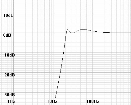
| Figure 6: Frequency response for speaker and filter for input parameters f = 45Hz and q = 0.9 |
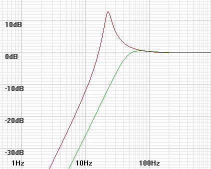 |
Figure 7: Combined frequency response for input parameters f = 45Hz and q = 0.9 |
 |
SPICE Simulation
Verify your design by running the SPICE model generated by the
program. Before doing so delete or comment out the non-SPICE
lines.| Figure 8: SPICE model generated by program for input parameters f = 45Hz and q = 0.9 |
| * filter simulation for input
parameters f = 45Hz and q = 0.9 v1 vin 0 dc 0 ac 1 sin 0 1V 1kHz rs vin 0 100k * filter emulating speaker response c3 vin c3c4 0.1u c4 c3c4 c4r4 0.1u r3 e2out c3c4 19648.8 r4 c4r4 0 63662 e2 e2out 0 c4r4 0 1 * electonic equalizer filter c1 e2out c1c2 0.1u c2 c1c2 c2r2 0.1u r1 e1out c1c2 8138.78 r2 c2r2 0 627452 e1 e1out 0 c2r2 0 1 * rl e1out 0 100k .end .control ac dec 30 1 100 plot db(e1out) db(e2out) db(e1out/e2out) .endc |
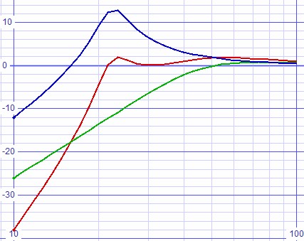
| Figure 9: SPICE plot of speaker, filter, and combined responses.. |
 |
Round the resistors to 1% values and reverfiy the simulation.
| Figure 10: Same SPICE model with resistors rounded to 1% values. |
| * filter simulation for input
parameters f = 45Hz and q = 0.9 v1 vin 0 dc 0 ac 1 sin 0 1V 1kHz rs vin 0 100k * filter emulating speaker response c3 vin c3c4 0.1u c4 c3c4 c4r4 0.1u r3 e2out c3c4 19648.8 r4 c4r4 0 63662 e2 e2out 0 c4r4 0 1 * electonic equalizer filter c1 e2out c1c2 0.1u c2 c1c2 c2r2 0.1u r1 e1out c1c2 8.06k r2 c2r2 0 634k e1 e1out 0 c2r2 0 1 * rl e1out 0 100k .end .control ac dec 30 1 100 plot db(e1out) db(e2out) db(e1out/e2out) .endc |
| Figure 11: SPICE plot of speaker, filter, and combined responses, resistors rounded to 1% values.. |
 |
Determining speaker parameters
The difficullty in designing such a fixed filter is in knowing the
required speaker specifications to some degree of precision. If
graphs of the speaker's frequency response are available the desired
parameters can be obtained by inspection. Note that away from the
resonant frequency the responses approach a straight line, a horizontal
one in the passband and a diagonal one in the stopband of slope
12dB/octave or 40dB/decade. These ideal response lines are called
asymptotes. If the passband asymptote and that of the stopband
are extended to where they intersect this intersection represents the
resonant frequency. Then if the actual magnitude response level
at that frequency is noted then that level represented in linear terms
is the same as the quality factor. Since the graph is certain to
show the magnitude in decibels rather than linear. It is
necessary to calculate the linear magnitude from the formula in equation 15 below.| (15) |
Qspeaker = 10 |
(magnitudedB(f0)
/
20) |
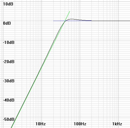
In figure 12 below the asymptotes cross at 40Hz giving the apparent resonant frequency. Then inspection shows the response at that frequency at ≈ –0.5. Then calculations yield Q.
| (15) |
Qspeaker = 10 |
(–0.5dB / 20) |
= 0.9441 |
Since the magnitude is close to the asymptote away from the resonant frequency, examining the frequency where the response falls to –40dB can also help. Then the resonant frequency is 10 times higher by knowing the asymptote slope of 40dB/decade.
| Figure 12: 2nd-order highpass plot showing how asymptotes cross at resonant frequency. |
 |
|
|
Conclusion
It is possible that other second-order highpass filter topologies could be used. Perhaps they could be shown at another time.|
|
1See related articles Butterworth Filter
Synthesis and Chebychev
Filter
Synthesis.
2Hardware design calculations derived
from:
Authur
B. Williams and Fred J. Taylor, Electronic Filter Design Handbook,
McGraw-Hill, New York, 1988.
Document History
January 14, 2017 Created.
January 14, 2017 Added missing last curly brace not copied with
program and added mention of use of SPICE Opus.
January 14, 2017 Added input for user to input his own C1/C2
choice to program.
March 21, 2017 Added section Determining
speaker
parameters.