Chebychev Filter Synthesis

Introduction

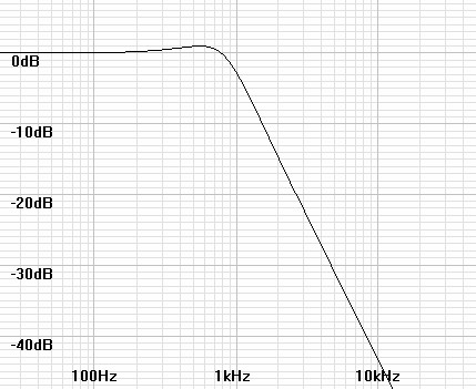
It is often desirable to design filters of higher than first order to some desirable specification such as flattest frequency response, sharpest cutoff, or linear phase. the last article of this type showed how Butterworth filters were synthesized. Next in order is the Chebychev filter.

Figure 1: Magnitude plot of 2nd order lowpass Chebychev filter.	Figure 2: Magnitude plot of 3rd order lowpass Chebychev filter.

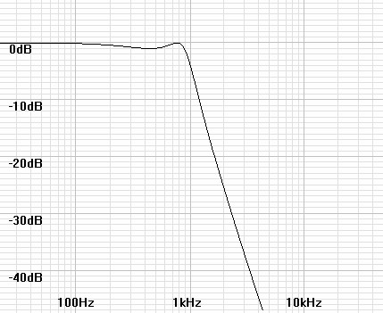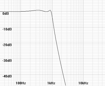
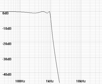
Figure 3: Magnitude plot of 4th order lowpass Chebychev filter.	Figure 4: Magnitude plot of 5th order lowpass Chebychev filter.

Synthesis of poles

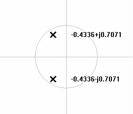
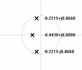
Like the Butterworth filter the mathematics for Chebychev synthesis begins with designing a pole plot. First Butterworth poles are created in the left half plane of the s-domain on the unit circle, then altered to an ellipse the multiplying by constants representing the filter specifications. Figures 5-8 show Chebychev pole plots from 2nd to 5th order.

Figure 5: S-domain plot of 2nd order lowpass Chebychev poles.	Figure 6: S-domain plot of 3rd order lowpass Chebychev poles.

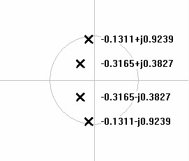
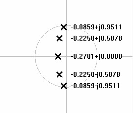
Figure 7: S-domain plot of 4th order lowpass Chebychev poles.	Figure 8: S-domain plot of 5th order lowpass Chebychev poles.

First calculate Butterworth poles for the desired order of filter. For N stages i to N the pole angles are calculated by:

(1)

θ_pole-i = 90° +

180° × (2i – 1)

Here however the angles of the poles is not sufficient. Therefore it is necessary to specify the poles in rectangular complex form.

(2)

α_i + jβ_i= cos(θ_pole-i) + jsin(θ_pole-i)

Perform the Chebychev conversion by multiplying the real part of each pole by a constant.

(3)

α_i' + jβ_i' = k_cheb⋅α_i + jβ_i

The Chebychev constant is calculated as follows.

(4)

ε =

10^{decibel-ripple/10} – 1

(5)

A =

sinh^-1

(6)

k_cheb = tanh(A)

Multiplication by the c alone specifies the design relative to its -3dB point. To specify it by its ripple cutoff, the entire pole must be multiplied by another constant as well.

(7)

α_i' + jβ_i' = k_ripple(k_chebα_i + jβ_i)

Where the constant is calculated as

(8)

k_ripple = cosh(A)

This is a equivalent to the following calculation.

(9)

α_i' + jβ_i' = sinh(A)⋅α_i + jcosh(A)⋅β_i

Convert poles to polar form ω_i∠θ_i.

(10)

ω_i = |α_i' + jβ_i'| =

α_i'² + β_i'²

(11)

θ_i = tan^-1

β_i'

α_i'

Highpass transformation

This point the filter is lowpass of frequency 1 rad/s. If a highpass filter is required it is better to do the transform before frequency scaling. For each pole ω_i∠θ_i invert the magnitude around a frequency of 1rad/s as follows.

(12)

ω_i-hp =

ω_i-lp

Deriving stage parameters from pole plot

It remains only to scale the magnitude to the desired frequency and calculate Q from θ_i.

(13)

f_stage-i =

ω_i × f_3dB

(if designed relative to 3dB cutoff.)

(14)

f_stage-i =

ω_i × f_{ripple--cutoff}

(if designed relative to ripple cutoff.)

It is acceptable to ignore the multiplying of mixed frequency units at this point because the initial frequencies are only relative. It is only when given a complete circuit specified to a certain frequency that units have to be accounted.

(15)

Q_stage-i =

2|cos(θ_i)|

Example

Show synthesis of 5th-order highpass Chebychev at 20Hz.

First, calculate pole angles for 5th order lowpass Butterworth filter according to equation 1.

θ_pole-1 = 90° +

180° × (2(1) – 1)

2(5)

θ_pole-1 = 90° +

180° × 1

θ_pole-1 = 90° + 18° = 108°

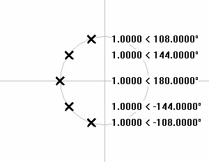
Continuing as above, each pole is 180/N° or 36° from the previous, thus creating the following sequence of remaining angles.

θ_pole-2 = 144°, θ_pole-3 = 180°, θ_pole-4 = 216°, and θ_pole-5 = 252°

Figure 9: Polar plot of 5th order lowpass Butterworth poles

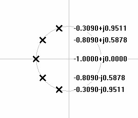
Now plot those angles onto the unit circle in rectangular complex form according to equation 2. The first pole calculates:

α_i + jβ_i = cos(108°) + jsin(108°) = –0.3090 + 0.9511

The remaining poles calculate to the values shown in the plot of figure 10 below.

Figure 10: Rectangular plot of 5th order lowpass Butterworth poles.

Begin the Chebychev transformation by calculating the Chebychev constant per equations 4-6.

(4)

ε =

10^1dB/10 – 1

10^0.1 – 1

1.258925^? – 1

0.258925

= 0.508847

(5)

A =

sinh^-1

0.508847

= 0.285595

(6)

k_cheb = tanh(0.285595) = 0.278076

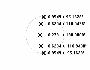
Multiply the real part of each Butterworth pole by k_cheb to give the lowpass Chebychev pole plot.

Figure 11: Rectangular plot of 5th order lowpass Chebychev poles.

Convert poles to polar form useful for highpass transformation and calculation of stage parameters by equations 10 and 11.

Figure 12: Polar plot of 5th order lowpass Chebychev poles.

Execute highpass transformation by taking the reciprocal of the magnitude of each pole.

Figure 13: Polar plot of 5th order highpass Chebychev poles.

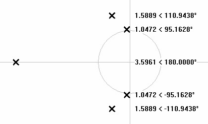Calculate stage parameters from pole values. First scale frequencies from magnitude for pole 1 (representing its conjugate as well)..

(13)	f_stage-1 = ω₁ × f_3dB = 1.0472 × 20Hz = 20.944Hz

Then calculate its Q from its angle.

(15)

Q_stage-1 =

2|cos(θ₁)|

2|cos(95.1628°)|

= 5.556422

Calculations from the remaining poles give a final result.

Stage	Frequency	Quality Factor
1	20.944Hz	5.556
2	31.778Hz	1.399
3	71.9229Hz	first order

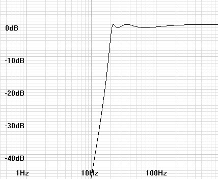
Figure 14: Frequency response of designed filter.

Hyperbolic functions

In case your calculator or programming library doe not have hyperbolic functions these are how they are calculated.

(16)

sinh(x) =

e^x – e^-x

(17)

cosh(x) =

e^x + e^-x

(18)

tanh(x) =

e^x – e^-x

e^x + e^-x

(19)

sinh^-1(x) =

^/ln

x^?+

x² + 1

¹The basis for most of the calculations in this article are from notes taken long ago from (as best I can remember):
Zverev, A. I., Handbook of Filter Synthesis, John Wiley and Sons, New York, 1967.

Document History
December 31, 2016 Created.