Butterworth Filter Synthesis

Introduction

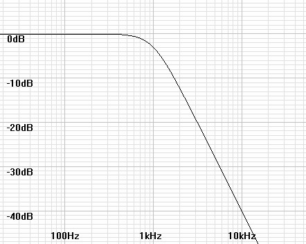
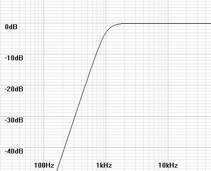
It is often desirable to design filters of higher than first order to some desirable specification such as flattest frequency response, sharpest cutoff, or linear phase. Here it is useful to begin by showing how a filter is designed for flattest frequency response, that is extended without ripple as flat as possible toward the –3dB point. The Butterworth filter meets this requirement and is usually called a maximally flat response filter. Figures 1–4 show these filters increase in sharpness of cutoff as order goes from two to five.

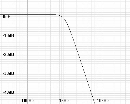
Figure 1: Magnitude plot of 2nd order Butterworth filter.	Figure 2: Magnitude plot of 3rd order Butterworth filter.

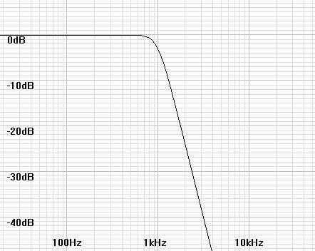
Figure 3: Magnitude plot of 4th order Butterworth filter.	Figure 4: Magnitude plot of 5th order Butterworth filter.

Synthesis of poles

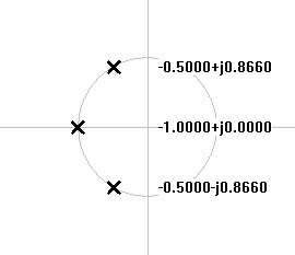
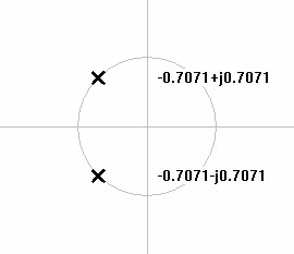
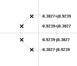
The mathematics for Butterworth synthesis begins with designing a pole plot. The pole specification arranges the poles in the left half-plane spaced evenly on a circle equidistant from the origin of the s-domain and centered symmetrically about the real axis. Where N is the order of the filter, the angle spacing between adjacent poles is 180°/N. Figures 5-8 show Butterworth pole plots from 2nd to 5th order.

Figure 5: S-domain plot of 2nd order lowpass Butterworth poles.	Figure 6: S-domain plot of 3rd order lowpass Butterworth poles.

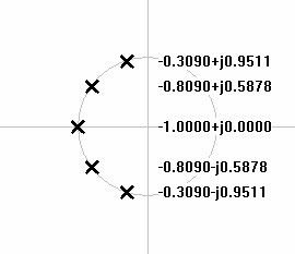
Figure 7: S-domain plot of 4th order lowpass Butterworth poles.	Figure 8: S-domain plot of 5th order lowpass Butterworth poles.

For N stages i to N the pole angles are calculated by

(1)

θ_pole-i = 90° +

180° × (2i – 1)

Deriving stage parameters from pole plot

If the Butterworth filter is implemented as an active filter, the design will consist of separate stages in sequence. Complex pole pairs will combine into second order stages. Any real pair will be represented by a simple first order stage. The fact that the poles are all equidistant from the origin of the s-domain plot corresponds to another property of the filter that all of the stages of the filter have the same resonant frequency (or cutoff frequency for any first order stage required by an odd order filter.). The final filter has a –3dB at that same frequency. It is really only necessary to specify the quality factor (Q) for each second order stage calculated from the angle of one of its complex poles. Equation 2 derives the Q for each angle θ calculated from equation 1.

For integer i ≤ N/2

(2)

Q_stage-i =

2|cos(θ_pole-i)|

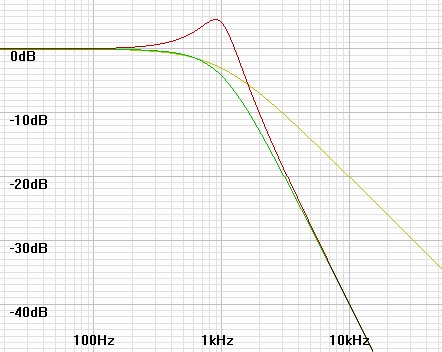
The individual magnitude responses of the sequential stages multiply (add in a decibel plot) to give the final response. Figure 9 below plots the magnitude response of each stage in a 5th order filter before multiplying to produce the plot of figure 4 above.

Figure 9: Magnitude plot of 5th order Butterworth filter stages.

Highpass transformation

Usually the first design step creates a lowpass filter, then if a highpass filter is desired the defining frequency of each stage is inverted geometricall around the overall -3dB frequency as calculated in equation 3. In this case, because all defining frequencies are the same as the cutoff, no change in frequency results. Then the hardware stages will be lowpass or highpass as the overall system is.

(3)

f_{pole-highpass} =

f_3dB-system²

f_pole-lowpass

Figure 10: Magnitude plot of 3rd order Butterworth filter.

Example

Calculate pole angles for 5th order filter

θ_pole-1 = 90° +

180° × (2(1) – 1)

2(5)

θ_pole-1 = 90° +

180° × 1

θ_pole-1 = 90° + 18° = 108°

Continuing as above, each pole is 180/N° or 36° from the previous, thus creating the following sequence of remaining angles.

θ_pole-2 = 144°, θ_pole-3 = 180°, θ_pole-4 = 216°, and θ_pole-5 = 252°

Now calculate quality factors. Where a pole is one of a complex conjugate (that is, that it is mirrored across the horizontal axis) only one of them has to be calculated.

Q_stage-1 =

2|cos(108°)|

Q_stage-1 =

2|-0.309017)|

= 1.61803

Continuing the same calculation gives Q values for the remaining stages.

Q_stage-2 = 0.61803 and Q_stage-3 = 0.5

The Q for stage three is only given for completeness, as it is known from examination that 180° represents a first-order stage. The remainder of poles are complex conjugates of ones already calculated for stages 1 and 2.

Hardware implementation

All filters with only poles – Butterworth, Chebychev, Bessel, and others – use the same sort of hardware of which there are multiple variations. Therefore hardware implementation is another subject.

Document History
November 18, 2016 Created.
November 25, 2016 Added highpass bode plot and example of calculation of pole angles and Qs.