Home  │ Audio Home Page

Copyright © 2010 by Wayne Stegall
Updated July 21, 2010.  See Document History at end for details.
Spice verfied.

Simple DC Servos

Introduction

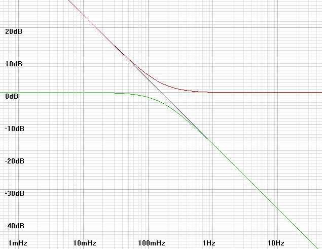
The hope of direct coupling some desireable audio circuits may be challenged by high DC offset, perhaps due to compromises made to gain some other desireable outcome.  Adding or increasing DC feedback is necessary here.  Second order servos are often used because a second passive pole is desired to decouple the typical op-amp integrator from the signal path.  Second order servos, however, require carefull juggling of gain and phase shift factors to prevent subsonic oscillation.  A simple integrator stage would do, but most would find the connection of the op-amp output into the signal path disagreeable.  Here I suggest adding to the integrator a zero matching and cancelling the pole of the second stage to create a two stage first order servo.  With a constant servo phase shift of -90°, design can proceed without worry of oscillation at all.

Figure 1:  Bode plot shows how response of integrator with zero (red plot) adds to that of the second stage lowpass pole (green plot) to create a first order integrator response (connecting black plot).

Figure 2:  Non-inverting and inverting two stage first order servos.

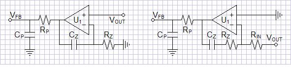A disadvantage of this design is that the output signal is present in full with boosted DC error signal at output of the integrator awaiting suppression by second stage.  Biasing of the servo must allow headroom for AC component.

Calculations

The final highpass pole will be at the frequency where |β_servo| = |β_global|.  β is feedback factor or gain of feedback loop.
To prove this assertion and give you useful servo equations, include both feedback factors in the closed-loop feedback gain equation:

AV-CL =

AV-OL 1+AV-OLβ

=

AV-OL 1+AV-OL(βglobal+βservo)

If the loop gain A_V-OLβ >> 1 (usually met, except in low gain circuits) then the ideal gain equation becomes:

AV-CL =

AV-OL 1+AV-OL(βglobal+βservo)

=

AV-OL AV-OL(βglobal+βservo)

=

1 (βglobal+βservo)

At the servo highpass pole, |β_servo| = |β_global| but their phases are 0º and -90º respectively.  The gain now becomes:

AV-CL =

1 βglobal - jβservo

=

1 βglobal(1 - j)

, (j here is a vector number with a 90º degree direction)

1/(1 - j) in polar terms is 0.7071<45º the -3dB response of a first order highpass filter.
These equations ideally include the high-frequency effects that require compensation calculations, but here are used only as they affect servo operation.

The servo feedback factor is inversely proportional to frequency.  Where ω = 2πf = 1/T and ω_pz is the frequency of the integrator zero and of the second stage pole:

βservo = βservo0

ωpz ω

= βservo0

fpz f

β_servo0 represents servo gain at ω_pz and is unity for the non-inverting circuit.  For the inverting circuit

βservo0 =

Rz Rin

You will have to multiply into β_servo0 any other gain factors you may add.  A likely example is the addition of a voltage divider before the integrator in a power amp where the direct output voltage would overdrive the op amp.

Exact calculations depend on the particular setup.  Refer to the example below for details.

Example

As an example I will add a non-inverting servo of this type to the voltage feedback amplifier of Musical Feedback Amplifiers.  It will function in this circuit to automatically bias the amplifier as well as reduce offset.  Offset will not be as low as it would be if servo was not acting to bias the ciruit as well, but it should still be good.  As a desirable side effect, driving the circuit bias will put the op-amp in class A operation, reducing the urge to use separate power supplies. 

The following circuit was unstable without compensation according to SPICE¹ modeling.  With dominant pole compensation of pole frequency >= 20kHz, it showed stable results.  I tried poles approaching 100kHz with good results also.  Its asymmetrical design should ensure even and odd harmonics for those with that preference.

The design proceeds as follows:

• Make transistor choices.  (I chose LSK170A JFETs and 2N3906 PNPs for these analyses, other choices would work well too.)
• Decide power supply voltages.
• Choose R_L (and R₁ and R₂ if used) for desired output impedance (in this case 1kΩ).
• Choose R_BE to set bias through Q₁.  Check Q₁ datasheet for a proper value here.
• Choose C_C for desired compensation pole frequency.  (Ordinarily this involves examining the loop gain (A_V-OLβ_global) in great detail, here SPICE should show whether our pole chosen for musical reasons will result in oscillation.)
• Simulate circuit in SPICE with reasonable R_S to negative power supply (R_S = V_SS/2I_D will do) and adjust compensation if needed.
• Choose servo break frequency of 159.155mHz for even 1sec time constant.
• Choose op-amp.  Any will do that will operate on the chosen power supply.  High DC gain and low output offset are desired, other parameters are less critical, bandwidth can be low.  The LF411 is often chosen for this sort of application.
• Calculate R_S to meet anticipated servo bias (i.e. terminated to -7.5V)
• Calculate R_2S and R_3S to drive desired servo bias from op-amp biased at output at 0V at reasonable current value within specs.
• Calculate feedback factors then calculate actual integrator pole and zero frequencies.
• From these calculate and choose remaining servo component values.
• Simulate and verify final circuit in SPICE.

Notes:
Output impedance in calculations is open-loop.  Closed loop output impedance will be reduced by the feedback factor (A_OL/A_CL).  Adding a small resistance (100Ω-1kΩ) on the output can give short circuit protection where an external cable is driven.

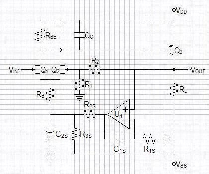
Figure 3:  Simplest voltage-feedback op-amp with non-inverting feedback network and DC servo.

Figure 3:  LSK170A SPICE model for reference

.MODEL LSK170A NJF + BETA   = 0.0378643       VTO    = -0.4025156      LAMBDA = 4.783719E-3        + IS     = 3.55773E-14      + RD     = 10.6565         RS     = 6.8790487                    + CGD    = 3.99E-11        CGS    = 4.06518E-11        + PB     = 0.981382        FC     = 0.5                + KF     = 0               AF     = 1

Amplifier Design and Compensation Procedure
Choose LSK170A JFETs and 2N3906 PNPs for these analyses
Choose power supplies as +-15V.

Z_OUT = R_L || (R₁ + R₂) = 1kΩ.
Choose R_L = 2kΩ, therefore R₁ + R₂ = 2kΩ.
For gain of 10, R₁ = 200Ω, R₂ = 1.8kΩ. (Ideal gain formula here is A_CL = 1 + R₂/R₁)
i_B-Q3 = -V_SS/(h_fe x Z_OUT) = 15/(100 x 2kΩ) = 75µA.
LSK170A has min I_DSS of 2.6mA, choose i_D = 2mA and calculate R_BE.
R_BE = v_be/(i_D - i_B-Q3) = 700mV/(2mA - 75µA) = 363.6363636Ω.
Round up to nearest standard 5% value:  R_BE = 360Ω.
r_b-Q3 = V_T/i_B-Q3 = 25mV/75µA = 333.3333333Ω. (V_T is the temperature dependent characteristic voltage of a PN junction, usually 25-26mV)
R_POLE = R_BE || r_b-Q3 = 360Ω || 333.3333333Ω = 173.0769231Ω
Calculate compensation capacitor for 20kHz dominant pole.

CPOLE =

1 2πfPOLERPOLE

=

1 2π x 20kHz x 173.0769231Ω

= 45.97809467nF

C_b = C_ibo + C_obo(A+1) = 10pF + 4.5pF(1kΩ/333.3333333Ω + 1) = 28pF (These from 2N3906 datasheet, multiplying C_obo by A+1 is the Miller effect)
C_C = C_POLE - C_b, because C_POLE >> C_b, C_C (approx.)= C_POLE = 45.97809467nF.
Choose standard value C_C = 47nF.
I_D  = 700mV/360Ω + 75µA = 2.01944mA
Calculate source output impedance r_s

rs =

1 gfs

=

1 2 x sqrt(knID)

=

1 2 x sqrt(37.8643mA/V2 x 2.01944mA)

= 57.1794Ω

Servo Design Procedure
Choose break frequency of 159.155mHz for even 1sec time constant.
Choose LF411 operational amplifier.

Want first stage of servo at 0V DC bias to drive C_2S of second stage to -7.5V
V_GS = V_T + sqrt(I_D/k_n) = -402.516mV + sqrt(2.01944mA/37.8643mA/V²) = -171.575mV
I_RS = 2 x I_D  = 4.03889mA
Calculate R terminated to -7.5V:
R_S = (7.5V + |V_GS|)/(i_D x 2) = (7.5V + 171.575mV)/4.03889mA = 1.89943kΩ.
Round down to nearest 5%.  Choose R_S = 1.8kΩ.
Calculate  R_2S for 10mA op-amp output:
R_2S = 7.5V/10mA = 750Ω.
R_3S = 7.5V/(10mA + 4.03889mA) = 534.23Ω.
Round up to nearest 5%.  Choose R_3S = 560Ω.
Now calculate to set servo break frequency.  Begin by calculating the feedback factors.

βglobal =

200Ω 1.8kΩ + 200Ω

= 0.1

Calculate additional drop in β_servo from that at integrator zero frequency (now presuming resistive voltage divider drop in second stage)

βservo-stage2 =

1.8kΩ || 560Ω 1.8kΩ || 560Ω + 750Ω

=

427.119Ω 427.119Ω + 750Ω

=

427.119Ω 427.119Ω + 750Ω

= 362.851m(V/V)

Preliminary SPICE evaluation indicates I underestimated additional drop (pole frequency was much lower than expected).  Proceed now on the basis of inserting the servo feedback at the Q₁ source rather than at the end of R_S.  Calculate additional drop due to voltage divider between R_S and r_s presuming voltage dividers are close to independent due to scale of impedances:

βatQ1Q2source =

rs RS || rs

=

57.1794Ω 1.8kΩ + 57.1794Ω

= 30.7883m(V/V)

β_servo0 =  β_servo-stage2 x β_atQ1Q2source = 362.851m(V/V) x 30.7883m(V/V) = 11.1716m(V/V)

Where ω = 2πf = 1/T:

βglobal = 0.1 = βservo =  βservo0

ωpz ω

=

βservo0 2πfhpTpz

Calculate servo pole/zero time constant from desired highpass break frequency:

Tpz =

βservo0 2πfhpβglobal

=

11.1716m(V/V) 2π x 159.155mHz x 0.1

= 111.716msec

R_{servo-pole-2ndst} = R_S || R_2S || R_3S = 1.8kΩ || 750Ω || 560Ω = 272.138Ω
C_2S = T_pz/R_{servo-pole-2ndst} = 111.716msec/272.138Ω = 410.512µF
Round to nearest standard 5% value:  Choose C_2S = 430µF.

Choose  R_1S = 330kΩ and calculate C_1S:
C_1S =  T_pz/R_1S = 111.716msec/330kΩ = 338.533nF
Round to nearest standard 5% value:  Choose C_1S =  330nF.

SPICE Results

Output offset = -13.3143µV
Frequency response:  0.17378Hz - 660.7kHz  +0,-3dB (Deviation of servo pole from chosen 0.159155Hz is negligible)
SNR = 109.875dB
Integrator output bias:  -1.33143V (You would want to trim R_2S or R_3S (and perhaps C_2S) if this value was too far from 0V)
Fourier analysis for vout @ 1kHz:
  No. Harmonics: 10, THD: 0.0296942 %, Gridsize: 200, Interpolation Degree: 1

Harmonic	Frequency	Magnitude	Phase	Norm. Mag	Norm. Phase
--------	---------	---------	-----	---------	-----------
0	0	0	0	0	0
1	1000	1.01354	-90.074	1	0
2	2000	0.000300274	-164.01	0.000296263	-73.939
3	3000	2.02959e-005	-73.348	2.00248e-005	16.7261
4	4000	9.88967e-007	11.5644	9.75756e-007	101.639
5	5000	3.507e-007	-179.5	3.46015e-007	-89.429
6	6000	1.89024e-007	74.622	1.86499e-007	164.696
7	7000	5.40419e-007	-6.6935	5.332e-007	83.3809
8	8000	1.70615e-007	-125.83	1.68336e-007	-35.755
9	9000	6.05319e-007	160.262	5.97233e-007	250.337

SPICE Model for circuit of figure 3¹.

¹Links to supporting SPICE models on this website: LSK170.txt, models1.txt

Document History
July 20, 2010  Created
July 21, 2010  Elaborated servo equations to better clarify integrator response.