Home  │ Audio Home Page

Copyright © 2016 by Wayne Stegall
Updated March 19, 2017.  See Document History at end for details.

Sealed-box Speaker Equalizer

Refer to preceding article Sealed-box Speaker Equalizer – Part 1 for preliminary background.

Introduction

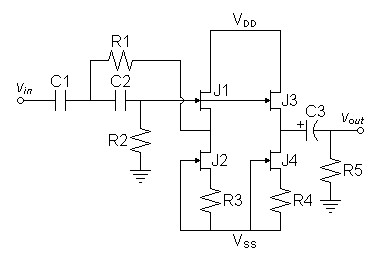
Because many audiophiles have an aversion to op amps, I decided to show how to design a discrete JFET speaker equalizer.  Figure 1 shows the resulting design using source-follower buffers.  Two buffers were used:  one for the feedback loop and another for the output.  This was to prevent any varying load on the output from altering the filter parameters.

Figure 1:  First schematic

Buffer design

I chose the 2N3819 n-channel JFET because is common and has reasonably good specifications like a 3nV/rtHz noise specification for some brands.  The MPF102 is similar if the specified part is not found.  The only element to calculate in the design of the buffer is the right value for the source resistor in the JFET current source to get the desired current bias.  I decided this simple calculation would give approximate midpoint bias.

(1)

Rs =

|VT| IDSS

For typical values of V_T = –3V and I_DSS = 10mA, R_s calculates to 300Ω.
For worst case values of V_T = –8V and I_DSS = 20mA, R_s calculates to 400Ω.
I chose the worst case and rounded R_s to the nearest 5% value of 390Ω.

Preliminary analysis

I expected to have to compensate R₁ for the output impedance of the buffer.  However because it might be reasonably thought that the low output impedance would have only a small effect on the result, I first simulated a design without compensation.

Figure 2: SPICE deck uncompensated for buffer output impedance.

* filter simulation for input parameters f = 45Hz and q = 0.9 vdd1 vdd 0 dc 15 vss1 vss 0 dc -15 v1 vin 0 dc 0 ac 1 sin 0 1V 1kHz rs vin 0 100k * filter emulating speaker response c3s vin c3c4 0.1u c4s c3c4 c4r4 0.1u r3s e2out c3c4 19648.8 r4s c4r4 0 63662 e2 e2out 0 c4r4 0 1 * electonic equalizer filter c1 e2out c1c2 0.1u c2 c1c2 c2r2 0.1u r1 j1s c1c2 8138.78 r2 c2r2 0 627452 j1 vdd c2r2 j1s 2N3819 j2 j1s vss j2s 2N3819 r3 j2s vss 390 j3 vdd c2r2 j3s 2N3819 j4 j3s vss j4s 2N3819 r4 j4s vss 390 c3 j3s vout 10u r5 vout 0 100k .model 2N3819 njf vto=-3.0 beta=1.3m .end .control ac dec 30 10 100 plot db(vout) db(e2out) db(vout/e2out) .endc

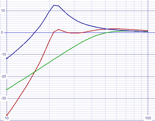
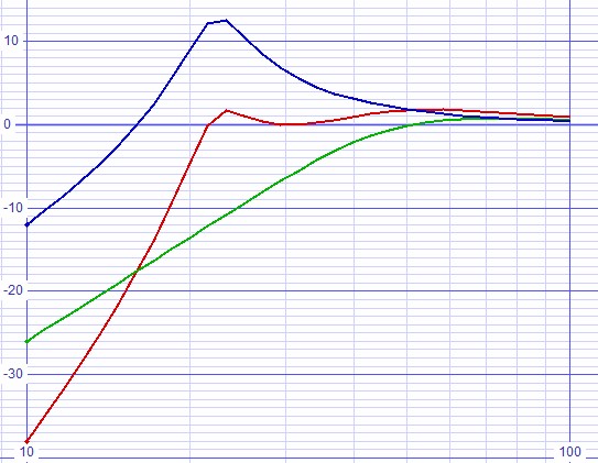
Figure 3: Bode plot uncompensated for buffer output impedance shows unequal ripple slightly over 0.5dB.

Analysis with compensation

Having established and imperfect uncompensated result, determine the output impedance of the JFET buffer.  Having a SPICE model at hand it is easiest to have SPICE give the desired value.  For this purpose, I used the transfer function analysis (tf).  Since tf is a DC analysis the capacitors in the circuit will both isolate the output impedance from other resistances in the circuit but also invalidate all the other results of the test.

Figure 4: SPICE determination of J1 output impedance.

SpiceOpus (c) 1 -> tf v(j1s) v1 SpiceOpus (c) 2 -> print all input_impedance = 1.000000e+005 output_impedance = 2.346907e+002 transfer_function = 0.000000e+000 SpiceOpus (c) 3 ->

Now it is only necessary to subtract the JFET output impedance from the design value to get the actual component value for R₁.

(2)	R1-component = R1-calculated – rs-j1

Figure 5: SPICE deck subtracting buffer output impedance from R1.

* filter simulation for input parameters f = 45Hz and q = 0.9 vdd1 vdd 0 dc 15 vss1 vss 0 dc -15 v1 vin 0 dc 0 ac 1 sin 0 1V 1kHz rs vin 0 100k * filter emulating speaker response c3s vin c3c4 0.1u c4s c3c4 c4r4 0.1u r3s e2out c3c4 19648.8 r4s c4r4 0 63662 e2 e2out 0 c4r4 0 1 * electonic equalizer filter c1 e2out c1c2 0.1u c2 c1c2 c2r2 0.1u * r1 = 8138.78 - 234.69 r1 j1s c1c2 7904.09 r2 c2r2 0 627452 j1 vdd c2r2 j1s 2N3819 j2 j1s vss j2s 2N3819 r3 j2s vss 390 j3 vdd c2r2 j3s 2N3819 j4 j3s vss j4s 2N3819 r4 j4s vss 390 c3 j3s vout 10u r5 vout 0 100k .model 2N3819 njf vto=-3.0 beta=1.3m .end .control tran 1u 0.1 0 1u fourier 1k vout ac dec 30 10 100 plot db(vout) db(e2out) db(vout/e2out) .endc

Now run the SPICE deck to show the new frequency response. 

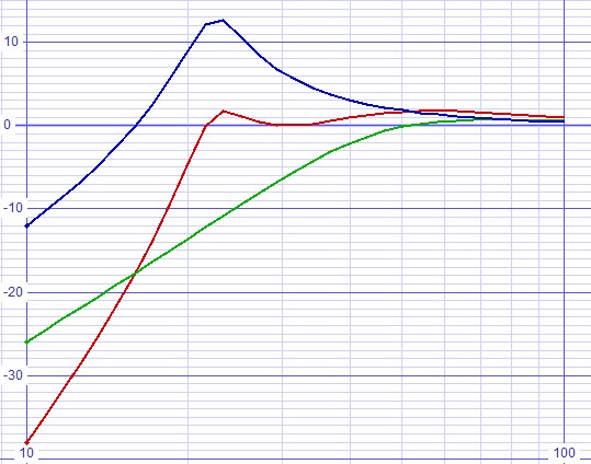
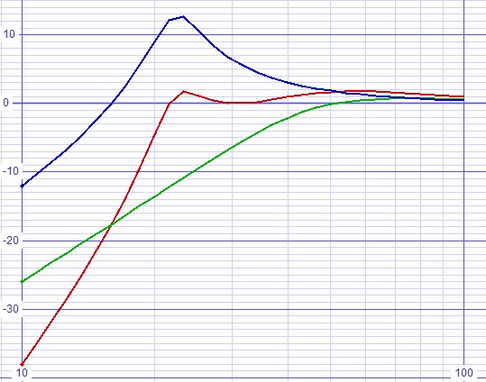
Figure 6: Bode plot compensated for buffer output impedance has equal ripple.

Input buffer adds another complication

At this point I realized that an actual finished circuit will have an input buffer to protect the equalization components from external alterations.  Instead of starting over again, I considered the analysis to this point still relevant and decided to continue on that basis.

Figure 7:  Schematic of filter with input buffer added.

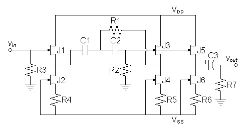Now adding an input buffer adds more design complication than the output impedance of the output buffers posed.  Instead of merely subtracting a simple value from the calculated one, the output impedance of the input buffer affects the equalization components in a more complicated way.  I expect both f₀ and Q of the filter to be lowered.

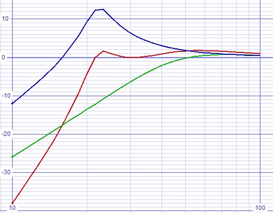
Figure 8: Bode plot uncompensated for input buffer output impedance shows a small amount of unequal ripple.

Facing a choice between calculating a new equalization model with an additional resistance added before C₁ or using a numerical iteration method, I remembered that a filter book recommended compensating LCR filters for stray circuit resistance (the of the inductor) by designing to circuit parameters altered slightly according to a certain formula.¹  I decided to use reasonable numerical approach of my own.  That is to design from parameters (guesses) then run a pole zero analysis in SPICE.  Then new values for the parameters are be calculated according the following formula.

(3)

valuenew-guess =

valueold-guess ×

valuetarget valuespice-result

This process is then repeated until the results converge to the desired specifications.

To this end I wrote another filter program generating a fully compensated SPICE deck.  Note constant ROJ came from the tf analysis run earlier and must be changed if you change the bias or specifications of the buffers.

Figure 9:  Code listing for filter program sbeqnjf.cpp:

#include <iostream> #include <complex> #include <stdio.h> #include <math.h> //#include <mathext.h> //include inverse hyperbolic functions. using namespace std; #define ORDER 4 #define sqr(x) ((x)*(x)) #define ROJ 234.69 int main(int argc, char* argv[]) {     int p, ret;     double qmin,f,q,f2,f3db,fripple,q2,thetap,pi,kcheby,A,epsilon,dbripple;     double fsf, c1c2, c1c2u, r1[2], r2[2];     complex <double> buttp[2], chebp[2];         double fmult, qmult;     pi = acos(-1);         fmult = 1.0;         qmult = 1.0;        // calculate first two poles of 4th order Butterworth     for(p=0;p<2;p++)     {         thetap = (pi/2.0)+(2.0*(p+1)-1.0)*pi/(2.0*(double)ORDER);         // cout << thetap*180.0/pi << endl;         buttp[p] = complex<double>(cos(thetap),sin(thetap));     }     qmin = abs(buttp[1])/(2.0*fabs(real(buttp[1])));     // get f and q from command line.     ret = 0;     if(argc == 4 || argc == 6)     {         ret = sscanf(argv[1],"%lg",&f);         if(ret)             ret = sscanf(argv[2],"%lg",&q);         if(ret)             ret = sscanf(argv[3],"%lg",&c1c2u);                 if(ret && argc == 6)                 {                     ret = sscanf(argv[4],"%lg",&fmult);         if(ret)                     ret = sscanf(argv[5],"%lg",&qmult);                 }     }     // else get them from input.     do     {         if(!ret)         {             cout << "Enter frequency, Q, and C1/C2 value in microfarads" << endl;             cin >> f >> q >> c1c2u;         }         if(q <= qmin)         {             cout << "Quality factor must be greater than " << qmin << endl;             // prevent command line operation from getting stuck             if(argc == 3)                 return -1;         }     } // loop back until q is correct     while(q <= qmin);     // Calculate existing Chebychev pole     chebp[1] = complex<double>(-1.0/(q*2.0),sqrt(1.0-sqr(-1.0/(q*2.0))));     chebp[1] *= complex<double>(imag(buttp[1])/imag(chebp[1]));     // Calculate design constants     kcheby = real(chebp[1])/real(buttp[1]);     A = atanh(kcheby);     epsilon = 1.0/sinh(A*ORDER);     dbripple = 10.0*log10(sqr(epsilon)+1.0);     f3db = f*abs(chebp[1]);     fripple = f3db*cosh(A);     // Calculate remaining Chebychev pole     chebp[0] = complex<double>(real(buttp[0] * kcheby),imag(buttp[0]));     q2 = fabs(0.5/cos(arg(chebp[0])));     f2 = f3db/abs(chebp[0]);     for(p = 0; p < 2; p++)         cout << "buttp[" << p << "] = (" << real(buttp[p]) << "," << imag(buttp[p]) << ")" << endl;     cout << endl;     for(p = 0; p < 2; p++)         cout << "chebp[" << p << "] = (" << real(chebp[p]) << "," << imag(chebp[p]) << ")" << endl;     cout << endl;     cout << "Filter frequency = " << f2 << endl;     cout << "Filter Q = "   << q2 << endl;     cout << "System dB ripple = " << dbripple << endl;     cout << "System -3dB frequency = " << f3db << endl;     cout << "System ripple frequency = " << fripple << endl << endl;         // adjust filter pole if necessary     if(argc == 6)     {         f2 *= fmult;         q2 *= qmult;         thetap = acos(-0.5/q2);         chebp[0] = polar(f3db/f2,thetap);         cout << "Request to scale filter: f by " << fmult << " and q by " << qmult << endl;         cout << "Filter frequency = " << f2 << endl;         cout << "Filter Q = "   << q2 << endl;         p = 0;         cout << "chebp[" << p << "] = (" << real(chebp[p]) << "," << imag(chebp[p]) << ")" << endl << endl;     }     // calculate unity gain Sallen and Key hardware.     c1c2 = c1c2u * 1.0e-6;     fsf = 1.0/(2*pi*f3db*c1c2);     for(p = 0; p < 2; p++)     {         r1[p] = -real(chebp[p])*fsf;         r2[p] = -norm(chebp[p])/real(chebp[p])*fsf;     }     // output SPICE model     cout <<    "* filter simulation for input parameters f = " << f << "Hz and q = " << q <<endl;     cout << "* Filter scaled: f by " << fmult << " and q by " << qmult << endl;     cout << "vdd1 vdd 0 dc 15" << endl \         << "vss1 vss 0 dc -15" << endl \     << "v1 vin 0 dc 0 ac 1 sin 0 1V 1kHz" << endl \     << "rs vin 0 100k" << endl \     << "* filter emulating speaker response" << endl \     << "c3s vin c3c4 " << c1c2u << "u" << endl \     << "c4s c3c4 c4r4 " << c1c2u << "u" << endl \     << "r3s fltrin c3c4 " << r1[1] << endl \     << "r4s c4r4 0 " << r2[1] << endl \     << "e2 fltrin 0 c4r4 0 1" << endl \     << "* electonic equalizer filter" << endl \         << "r3 fltrin 0 47k" << endl \         << "j1 vdd fltrin j1s 2N3819" << endl \         << "j2 j1s vss j2s 2N3819" << endl \         << "r4 j2s vss 390" << endl \     << "c1 j1s c1c2 " << c1c2u << "u" << endl \     << "c2 c1c2 c2r2 " << c1c2u << "u" << endl \         << "* r1 = " << r1[0] << " - " << ROJ << endl \     << "r1 j3s c1c2 " << r1[0]-ROJ << endl \     << "r2 c2r2 0 " << r2[0] << endl \         << "j3 vdd c2r2 j3s 2N3819" << endl \         << "j4 j3s vss j4s 2N3819" << endl \         << "r5 j4s vss 390" << endl \         << "j5 vdd c2r2 j5s 2N3819" << endl \         << "j6 j5s vss j6s 2N3819" << endl \         << "r6 j6s vss 390" << endl \         << "c3 j5s vout 10u" << endl \         << "r7 vout 0 100k" << endl \         << ".model 2N3819 njf vto=-3.0 beta=1.3m" << endl \         << ".end" << endl \         << ".control" << endl \         << "pz c4r4 0 c2r2 0 vol pol" << endl \         << "print all" << endl \         << "*tran 1u 0.1 0 1u" << endl \         << "*fourier 1k vout" << endl \         << "ac dec 30 10 100" << endl \         << "plot db(vout) db(fltrin) db(vout/fltrin)" << endl \         << ".endc" << endl << endl;     return 0; }

Note that if you compile the program in Visual C++ 6.0 you will have to include your own library of inverse hyperbolic functions.  Linux has them already and other compilers perhaps as well.

To compile in Linux enter:
g++ <c++ filename> -lm -o <executable filename>

If you named the program sbeq.cpp enter:
g++ sbeqnjf.cpp -lm -o sbeqnjf

Make the program executable:
chmod +x sbeqnjf

Then run it.  Filter compensation multipliers are only programmed to be input from the command line.  So this is the proper command to run the program to send output to a file for obtaining and running the SPICE model.

./sbeqnjf <spkr resonant freq> <spkr Q> <C1/C2 value in microfarads> <f multiplier> <q multiplier > <output file>

i.e.
./sbeqnjf 45.0 0.9 0.1 1.04 1.1 > sbeqnjf.txt

The optimization was carried out in a spreadsheet by the following procedure.

• The initial frequency and q guesses are those of the initial design goals calculated from the speaker parameters.  The initial frequency and q design goals are repeated as constants in the last columns to make calculations easier.
  
• each iteration calculates new guesses from the previous iteration's SPICE results.  (Note the pole taken from SPICE is the more positive of the one in a complex conjugate pair.)
• The program is run to get a SPICE deck compensated for the current iteration.
• SPICE is run and the pole values are copied to the spreadsheet for that iteration.
• If necessary copy current iteration to next to copy formulas.  New guesses and multipliers will appear correct only to await insertion of SPICE results.

Figure 10: Spreadsheet managing numerical iteration calculations.

Calculated Guesses Program Input SPICE Results Constants iteration f guess q guess fmult qmult pole real pole imag f result q result 1 22.2715 4.39016 1 1 -16.16124 138.9736 22.26739031 4.328570693 22.2715 4.39016 2 22.27561045 4.452625634 1.000184561 1.014228555 -15.94081 139.0254 22.27155569 4.389247205 22.2715 4.39016 3 22.27555475 4.45355161 1.00018206 1.014439476 -15.9375 139.0255 22.2715115 4.39015008 22.2715 4.39016 4 22.27554325 4.453561673 1.000181544 1.014441768 -15.93745 139.0254 22.27149478 4.390160558 22.2715 4.39016 5 22.27554847 4.453561107 1.000181778 1.014441639 -15.93745 139.0254 22.27149478 4.390160558 22.2715 4.39016

Iterations 4 and 5 having the same SPICE results stops the iteration.  I think the default precision of the c++ cout() function for double values used to print the SPICE model brought the iteration to a halt this way.

If you want to use the same spreadsheet, the only input cells are the guesses of iteration 1 and pole results returned from SPICE.  The remaining cells contain calculations.

Download Excel spreadsheet.

Figure 11: Fully optimized SPICE deck from iteration 5.

* filter simulation for input parameters f = 45Hz and q = 0.9 * Filter scaled: f by 1.00018 and q by 1.01444 vdd1 vdd 0 dc 15 vss1 vss 0 dc -15 v1 vin 0 dc 0 ac 1 sin 0 1V 1kHz rs vin 0 100k * filter emulating speaker response c3s vin c3c4 0.1u c4s c3c4 c4r4 0.1u r3s fltrin c3c4 19648.8 r4s c4r4 0 63662 e2 fltrin 0 c4r4 0 1 * electonic equalizer filter r3 fltrin 0 47k j1 vdd fltrin j1s 2N3819 j2 j1s vss j2s 2N3819 r4 j2s vss 390 c1 j1s c1c2 0.1u c2 c1c2 c2r2 0.1u * r1 = 8021.46 - 234.69 r1 j3s c1c2 7786.77 r2 c2r2 0 636398 j3 vdd c2r2 j3s 2N3819 j4 j3s vss j4s 2N3819 r5 j4s vss 390 j5 vdd c2r2 j5s 2N3819 j6 j5s vss j6s 2N3819 r6 j6s vss 390 c3 j5s vout 10u r7 vout 0 100k .model 2N3819 njf vto=-3.0 beta=1.3m .end .control pz c4r4 0 c2r2 0 vol pol print all *tran 1u 0.1 0 1u *fourier 1k vout ac dec 30 10 100 plot db(vout) db(fltrin) db(vout/fltrin) .endc

Now run final SPICE deck for bode plot.

Figure 12: Bode plot from fully optimized SPICE deck.

Round the filter components to 1% values (only affects R₁ and R₂) and do SPICE analyses.

Figure 13: Fully optimized SPICE deck from iteration 5 with filter components rounded to standard 1% values.

* filter simulation for input parameters f = 45Hz and q = 0.9 * Filter scaled: f by 1.00018 and q by 1.01444 vdd1 vdd 0 dc 15 vss1 vss 0 dc -15 v1 vin 0 dc 0 ac 1 sin 0 1.41421V 1kHz rs vin 0 100k * filter emulating speaker response c3s vin c3c4 0.1u c4s c3c4 c4r4 0.1u r3s fltrin c3c4 19648.8 r4s c4r4 0 63662 e2 fltrin 0 c4r4 0 1 * electonic equalizer filter r3 fltrin 0 47k j1 vdd fltrin j1s 2N3819 j2 j1s vss j2s 2N3819 r4 j2s vss 390 c1 j1s c1c2 0.1u c2 c1c2 c2r2 0.1u * r1 = 8021.46 - 234.69 r1 j3s c1c2 7.87k r2 c2r2 0 634k j3 vdd c2r2 j3s 2N3819 j4 j3s vss j4s 2N3819 r5 j4s vss 390 j5 vdd c2r2 j5s 2N3819 j6 j5s vss j6s 2N3819 r6 j6s vss 390 c3 j5s vout 10u r7 vout 0 100k .model 2N3819 njf vto=-3.0 beta=1.3m .end .control pz c4r4 0 c2r2 0 vol pol print all tran 1u 0.1 0 1u fourier 1k vout ac dec 30 10 100 plot db(vout) db(fltrin) db(vout/fltrin) .endc

Figure 14: Bode plot from fully optimized SPICE deck with filter components rounded to standard 1% values.

Figure 15:  Spice distortion results from fourier analysis for 1kHz

Fourier analysis for vout:   No. Harmonics: 10, THD: 0.00156519 %, Gridsize: 200, Interpolation Degree: 1 Harmonic   Frequency   Magnitude   Norm. Mag   Percent   Decibels 1 1000 1.41212 1 100 0 2 2000 1.50533E-05 1.06601E-05 0.00106601 -99.44477443 3 3000 1.00149E-05 7.09215E-06 0.000709215 -102.9844418 4 4000 7.51394E-06 5.32106E-06 0.000532106 -105.4800369 5 5000 6.01313E-06 4.25824E-06 0.000425824 -107.4153973 6 6000 5.01309E-06 3.55006E-06 0.000355006 -108.9952861 7 7000 4.29918E-06 3.04449E-06 0.000304449 -110.329709 8 8000 3.76407E-06 2.66555E-06 0.000266555 -111.4842633 9 9000 3.34816E-06 2.37103E-06 0.000237103 -112.501259

Figure 14:  Noise analysis returns noise level of –115dB.

SpiceOpus (c) 1 -> noise v(vout) v1 dec 30 20 20k SpiceOpus (c) 2 -> print all inoise_total = 2.531133e-012 onoise_total = 2.974034e-012 SpiceOpus (c) 3 -> print db(onoise_total)/2 db(onoise_total)/2 = -1.15267e+002 SpiceOpus (c) 4 ->

Conclusions

None of the frequency plots looked bad.  I suppose perfection requires extra effort.

¹Authur B. Williams and Fred J. Taylor, Electronic Filter Design Handbook, McGraw-Hill, New York, 1988.  pp. 3-12–3-15, "Using Predistorted Designs".

Document History
March 18, 2017  Created.
March 19, 2017  Corrected incorrect filenames in program use instructions and added a brief paragraph on buffer design.