One-Bend Amplifier

Part 3: Modified circuit adds a predriver stage

Introduction

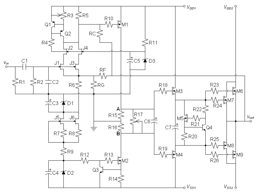
The quest for more slew rate seemed to suggest two paths: find lower capacitance power MOSFETs or add a predriver stage. Initial searches for faster transistor seemed a dead end, the IRF510 already had low capacitance for its abilities, and there were seemingly no lower capacitance output devices than the IRFP240 and IRFP9240 in a large plastic TO247 package. I was reluctant to add a predriver as well because I did not want to increase transfer curve complexity or lose the large phase margin that I apparently had. However, in the end I tried the predriver anyway.

Circuits

The predriver adds a buffer stage M3 and M4 to drive the 5000nF of total gate capacitance of the output transistors. After verifiying the circuit with resistor bias for the predriver, I decided that current bias consisting of M5, Q4, and their related components would be a more certain way to set the bias in the face of expected V_T variations in M3 and M4.

Figure 1: One-bend amplifier with predriver stage added.

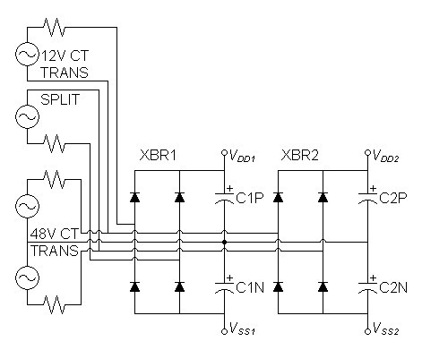
Adding the predriver circuit posed to take away 3 more volts of voltage headroom from the amplifier, an undesirable outcome. To compensate, I added another transformer to the power supply to raise the first, second, and predriver stage supplies above that of the output stage.

Figure 2: New power supply.

SPICE Results

SPICE model of amplifier
SPICE model of power supply

Power Bandwidth

Attempts to measure slew rate resulted in the difficulty of deciding which of the multiple slopes actually was representative. So I followed the recommendation of a TI technical document that suggested that power bandwidth be determined as the frequency at which the distortion rises to a certain level, possibly 1%. I experimented with the previous circuit to find powerbandwidth calculated from slew rate at about 1.2% distortion. By experiment, the power bandwidth of this circuit at approximately 1% distortion to be ≈ 45kHz.

Fourier analysis for vout:
No. Harmonics: 16, THD: 1.07739 %, Gridsize: 200, Interpolation Degree: 3

Harmonic	Frequency	Magnitude	Norm.Mag	Percent	Decibels
--------	---------	---------	---------	---------	---------
1	45000	21.0952	1	100	0
2	90000	0.161286	0.0076456	0.76456	-42.3318
3	135000	0.121504	0.00575976	0.575976	-44.7919
4	180000	0.0784135	0.00371712	0.371712	-48.5959
5	225000	0.0450847	0.0021372	0.21372	-53.4031
6	270000	0.0312462	0.00148119	0.148119	-56.5878
7	315000	0.0265608	0.00125909	0.125909	-57.9989
8	360000	0.0201131	0.000953441	0.0953441	-60.4141
9	405000	0.0138871	0.000658306	0.0658306	-63.6314
10	450000	0.0111787	0.000529915	0.0529915	-65.5159
11	495000	0.00993006	0.000470725	0.0470725	-66.5447
12	540000	0.00838333	0.000397404	0.0397404	-68.0154
13	585000	0.00711102	0.000337091	0.0337091	-69.4451
14	630000	0.00640845	0.000303786	0.0303786	-70.3487
15	675000	0.00572887	0.000271572	0.0271572	-71.3223

slew rate =

(peak) = 2πfv_pk = 2π × 45kHz × 21.0952V = 5.96453V/us

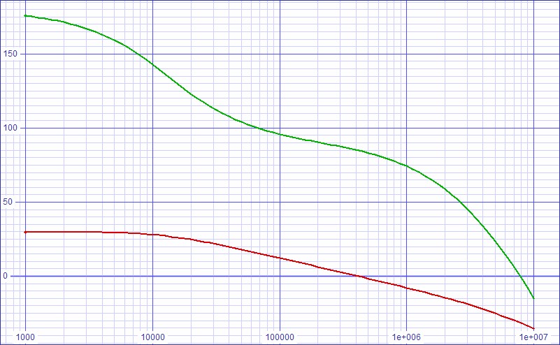
Stability Analysis

Figure 3: Loop gain shows dominant pole still greater than 10kHz and phase margin greater than 80 deg.

Distortion Results

Fourier analysis for vout @ 1kHz:
No. Harmonics: 16, THD: 0.0155797 %, Gridsize: 200, Interpolation Degree: 3

Harmonic	Frequency	Magnitude	Norm.Mag	Percent	Decibels

1	1000	21.1936	1	100	0
2	2000	0.00329427	0.000155437	0.0155437	-76.1689
3	3000	0.000223848	1.05621E-05	0.00105621	-99.525
4	4000	1.80022E-05	8.49415E-07	8.49415E-05	-121.418
5	5000	1.69424E-06	7.9941E-08	7.9941E-06	-141.945
6	6000	2.00519E-07	9.46127E-09	9.46127E-07	-160.481
7	7000	5.91641E-08	2.7916E-09	2.7916E-07	-171.083
8	8000	6.0557E-08	2.85732E-09	2.85732E-07	-170.881
9	9000	5.80361E-08	2.73837E-09	2.73837E-07	-171.25
10	10000	6.74031E-08	3.18035E-09	3.18035E-07	-169.951
11	11000	3.71128E-08	1.75113E-09	1.75113E-07	-175.134
12	12000	7.98147E-08	3.76598E-09	3.76598E-07	-168.482
13	13000	1.25026E-08	5.89922E-10	5.89922E-08	-184.584
14	14000	8.48198E-08	4.00214E-09	4.00214E-07	-167.954
15	15000	1.27269E-08	6.00508E-10	6.00508E-08	-184.43

Fourier analysis for vout @ 20kHz:
No. Harmonics: 16, THD: 0.00777008 %, Gridsize: 200, Interpolation Degree: 3

Harmonic	Frequency	Magnitude	Norm.Mag	Percent	Decibels

1	20000	21.1799	1	100	0
2	40000	0.00158615	7.48892E-05	0.00748892	-82.5116
3	60000	0.000403248	1.90392E-05	0.00190392	-94.407
4	80000	0.000165509	7.81444E-06	0.000781444	-102.142
5	100000	4.78777E-05	2.26052E-06	0.000226052	-112.919
6	120000	1.20349E-05	5.68224E-07	5.68224E-05	-124.91
7	140000	3.56298E-06	1.68225E-07	1.68225E-05	-135.482
8	160000	1.07192E-06	5.06101E-08	5.06101E-06	-145.915
9	180000	6.60838E-07	3.12012E-08	3.12012E-06	-150.117
10	200000	3.74125E-07	1.76642E-08	1.76642E-06	-155.058
11	220000	3.26926E-07	1.54357E-08	1.54357E-06	-156.229
12	240000	2.98762E-07	1.41059E-08	1.41059E-06	-157.012
13	260000	3.00341E-07	1.41805E-08	1.41805E-06	-156.966
14	280000	2.65863E-07	1.25526E-08	1.25526E-06	-158.025
15	300000	2.33183E-07	1.10096E-08	1.10096E-06	-159.165

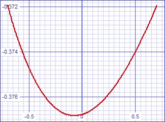
Transfer Error Curves

Figure 4: Small signal DC transfer error curve.	Figure 5: Large signal DC transfer error curve.

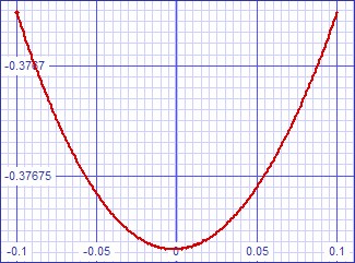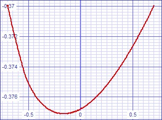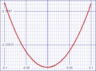
C7 removes the predriver from the transfer curves above a pole frequency set by C7 and the sum of the transconductances of M3 and M4. Above this pole there is a different ac transfer error curve.

Figure 6: Small signal AC transfer error curve.	Figure 7: Small signal AC transfer error curve.

If the feedback along the inner feedback loop is increased by reducing RC from 220kΩ to 100kΩ the AC transfer curves above become more symmetrical parabolas at the expense of somewhat greater overall distortion.

Conclusions

Since the gainclone amplifiers are popular, I examined their chipsets slew rates as a guideline. I have exceeded their minimum slew rate of 5V/µs but fallen short of their typical figures for this and the previous circuit. It would be a tossup to decide whether the extra predriver transistors are worth just an increase of slew rate from 5.3V/µs to nearly 6V/µs if fewer transistors is a virtue.
Eventually, I found some lateral MOSFETs with about ²/₃ the input capactance of the vertical MOSFETs more commonly available but they seemed to make no improvement perhaps because the substrate capacitance was higher.

Document History
June 9, 2012 Created.