Noise Shaping Music

DSD-like coding inside PCM digital audio content increases its resolution

Introduction

Perhaps you have heard that single rate DSD is the equivalent to 20 bit resolution at a sampling rate of 96kHz. Then imagine that the least significant bit (LSB)of a PCM recording could be modulated by a delta-sigma process to encode much or all of the resolution of a higher resolution signal. A CD resolution recording at 16bit/44.1kHz then by the same reasoning could have 20bits resolution encoded in its LSB below frequencies below 750Hz for a total of 35bits resolution diminishing back gradually to 15 bits at the higher frequencies where the noise has been shifted.

First order example

The simplest means to attempt this is first-order noise-shaping. This method reserves the remainder after the input has been rounded to fit in fewer bits and adds it back to the next sample before it is processed again in the same way.

Figure 1: Pseudocode for first-order noise-shaping

accumulator = 0;
while(input signal)
{
accumulator = accumulator + input;
// accumulator now sums previous remainder with new input
output = round(accumulator);
accumulator = accumulator - output;
// accumulator now contains remainder of round operation
}

This is roughly equivalent to an IIR (infinite impulse response) first-order analog-type lowpass digital filter for the LSB as defined by the following equation.

(1)	y_n = a₀x_n + b₁y_n-1

Here y is the output, x is input, n and n-1 are sample periods, and a₀ and b₁ are filter constants. a₀x_n represents rounded LSB energy and b₁y_n-1 represents remaindered LSB energy from the last sample. The way that the equation is interpreted is that the magnitude of b₁ relative to a₀ is related to exponential decay. A signal beginning at a magnitude of one decays exponentially to just b₁ in one sample period. Then that exponential decay is defined in terms of filter coefficients, sampling period, and lowpass break frequency.

(2)

–ω₀t

b₁

Where ω₀ = 2πf₀ and t = 1/f_s, the equation would become useful to calculate coefficients for other applications. Instead for this purpose definitions of our filter coefficients are implied by the process defined and the lowpass cutoff frequency is calculated instead.

(3)

–2πf₀

f_s

b₁

How are the filter coefficients inferred? When rounding occurred the average signal output in the LSB and the average remainder were both ½LSB. Where a₀ and b₁ = ½LSB the solution of the equation then proceeds.

(4)

–2πf₀

f_s

= 0.5

(5)

–2πf₀

f_s

= ln(0.5) = –0.693147

(6)

f₀ =

0.693147f_s

2π

= 0.110318f_s

If f_s = 44.1kHz

(7)	f₀ = 0.110318 × 44.1kHz = 4.86501kHz

The signal energy passed in the LSB is lowpass filtered at this break frequency, the noise instead is shaped by a highpass function complementary to the lowpass function that shapes inband portion of the LSB as shown in figure 2 below.

Figure 2: Envelope of shaped noise.

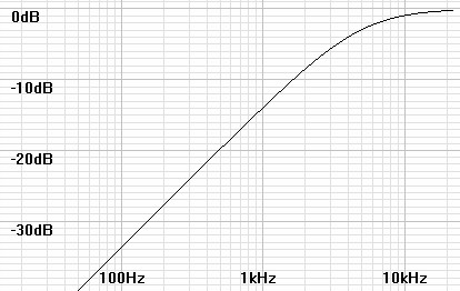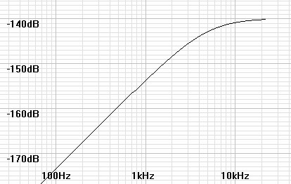
However the complementary highpass function determines only the shape of the noise response. The actual magnitude is scaled to retain all of the quantization noise that was originally distributed evenly. I have scaled the same noise shape to contain the –98dB total noise that unavoidable for this format.

Figure 3: Actual noise curve containing –98dB of noise in dB0FS(√Hz) units in the band below 22.05kHz.

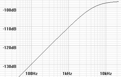
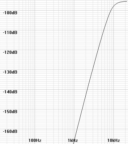
142.904dB corner

By multiplying the curve of figure 3 by the square root of the bandwidth figure 4 shows full bandwidth equivalent noise levels for comparing the shaped noise levels with the –98dB level of a flat noise curve. By inspection of figure 4 it appears that resolution improvements are gained which increase with decrease in frequency. Since a first order slope changes by 6dB/octave so too the resolution here in increases by one bit for every octave decrease in frequency. There is 16-bit resolution at about 7kHz, 20-bit at 250Hz, and off the graph 24-bit at 16Hz.

Figure 4: Noise curve adjusted to full bandwidth equivalent noise units for comparison.

Along with an increase in low frequency resolution, total perceived noise is also reduced by shifting the noise to higher frequencies where human hearing is less sensitive. If a-weighting – which is supposed to mimic the human ear's actual noise perception response – is multiplied with the noise curve and a noise integral done, a small improvement in perceived total noise is gained by the shaped noise of figure 3 over a flat noise curve of the same total noise.

	Unweighted	A-weighted
White noise	–98dB	–100.403dB
Shaped noise	–98dB	–101.534dB

Higher orders

The results of a first order modulator are modest but do not achieve the resolution improvements that the technique promises. However modulators of up to order seven are often used. No doubt these produce the desired results. In order to validate this idea I experimented to sort out what type of filter response would give an equivalent 24 bit resolution at low frequencies after noise shaping. I ended up adding a 4th order Butterworth filter at 9kHz to the same first order response already analyzed.

Figure 5: Actual noise curve containing –98dB of noise in dB0FS(√Hz) units in the band below 22.05kHz.

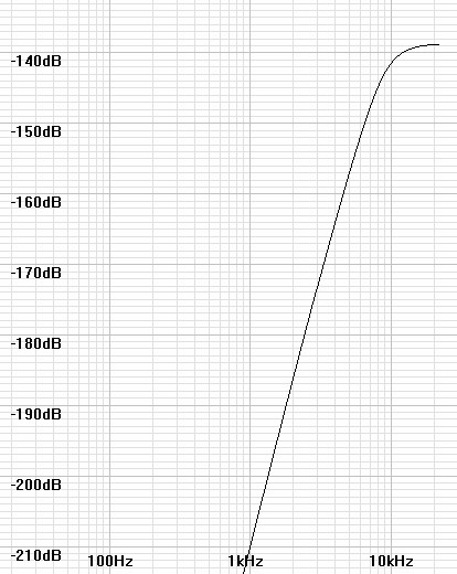Again, multiplying the graph by the square root of the bandwidth gives units comparable to full bandwidth noise so that resolution observations can be made. By inspection of figure 6 it remains true that resolution improvements are gained which increase with decrease in frequency. Since a first order slope changes by 6dB/octave so too the resolution here in increases by n bits bit for every octave decrease in frequency where n is the order of the filter slope at that point. There is 16-bit resolution at about 10kHz, 20-bit at 3.7kHz, and 24-bit at 1.8kHz. The result exceeds the 24 bit goal for many frequencies. Adding a-weighting gives a perceived total noise of –103.549dB, about a 3dB improvement over the –100.403dB perceived in the case of a flat noise floor.

Figure 6: Noise curve adjusted to full bandwidth equivalent noise units for comparison.

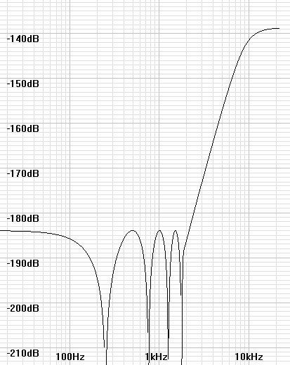
All of this optimism is curbed however when the filter is implemented. A fourth-order analog filter as graphed has phase shift far in excess of the 135º limit considered safe to insert in a feedback loop. In reality, a digital lowpass-filter of minimum group delay would simulate the Butterworth response. These filters have a small amount of passband ripple that when inserted into the feedback loop that become stopband ripple in the highpass noise curve. Then this limits how low the noise-shaping curve can go in the low frequencies and how much resolution can be obtained by careful reduction of ripple. In figure 7 below, I have drawn some ripple into the same graph to illustrate this point. The magnitudes shown are not necessarily those of an actual design.

Figure 7: Representative noise curve after implementing as digital filter.

History

As I understand it this process came later in the development of CD audio. The first CD recordings do not compare favorably with those that came later. This is likely because the PCM samples were only rounded, whether in the ADC itself or in the production process. The first improvement was the addition of dither to recordings. Dither added near LSB levels of white noise to music in advance of the ADC or to the digital content before reduction of bit resolution. In some cases 22.05kHz triangular wave dither was added. In any case, dither made the rounding process much more accurate on average over many samples thus benefiting linearity, especially at lower frequencies. The result was a great improvement in the sound of digital audio over the first recordings. Some credit dithering with producing the same vast increase in resolution that noise shaping does. However just adding an additional LSB level signal to the content allegedly reduces the signal to noise ratio to 93dB and is unlikely to produce the results of that only a controlled coding process could produce. Dither is likely credited this reputation because noise-shaping is often called dither as well – often as noise-shaped dither. Now recordings are either processed by dither, noise-shaping, or both, according to the discretion of those producing the music.

Final Remarks

This seems to mitigate CD's bad reputation to some extent, however the improvement in low and midrange resolution does not eliminate the CD resolution's high frequency defects.¹ For this reason, higher sampling rates still have value, not to mention giving somewhere to push the shaped noise out of the audio band. High bit resolution is still necessary, first as starting point to have resolution to encode by noise-shaping into lower bit resolutions. Noise-shaped CD content cannot be produced from 16 bit masters. Secondly, high resolution music and DACs have proven themselves to many audio enthusiasts. I think this is because noise shaping is unraveled in the upsampling filter of DACs and simultaneously rounded to the filter's bit resolution making it desirable for the bit resolution of the DAC to match or exceed that of the recording process. I think too that if these processes are performed internally by ADCs that 24 bit recordings may have more than 24 bits resolution, a quality that only a 32 bit DAC might preserve through its digital filters. (bold text newly added)

¹See related Article: Mathematical Consideration of Some of the Limitations of Digital Audio.
²See related Article: Digital Audio Formats
³See related Article: Delta-Sigma Modulators

Document History
April 3, 2015 Created.
April 4, 2015 Updated text and plots for more correct math.
May 27, 2015 Corrected equations 2 and 3 making pole only dependent on b₁; the a₀ coefficient only affects gain.
July 1, 2020 Added text to Final Remarks better clarifying why high bit resolution (32bit?) is desired in audio DACs..