 |
| Home │ Audio
Home Page |
Copyright © 2011 by Wayne Stegall
Updated January 6, 2011. See Document History at end for
details.
Computer verified.
Transfer Curve Shape and Distortion
Introduction
Investigated here is the common belief that the more bends a
transfer function has the worse the quality of its distortion.
Mathematical Analysis
To evaluate the assertion at hand it is necessary to choose suitable
mathematical models and methods. I chose to use sin/cos functions
as error functions added to a consistant linear function base (i.e. y = x - k(sin or cos)(m·x) ) in
order to have the same sort of distortion characteristic regardless
of the number of bends. I also decided to iterate for a value of
k in each case to give a total distortion of 0.01% to add another
element
of consistency. The transfer curve graphs are exaggerated as a
result because the actual transfer curves would still look very
flat. The methodology is to apply the transfer functions to one
cycle of a unity magnitude sine function then analyze the result with a
Fast Fourier
Transform.
The resulting Fourier series analysis gives the distortion breakdown by
harmonic.
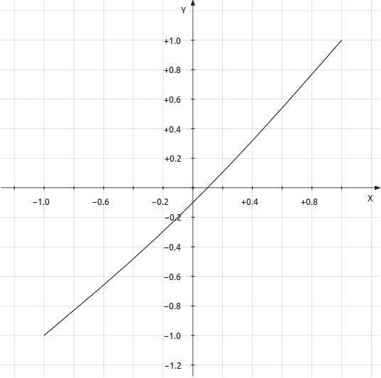
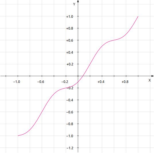
| Figure
1:
Transfer
Curve
1
—
y = x - k·cos(0.5π·x) |
|||||||||||||||||||||||||||||||||
 |
|||||||||||||||||||||||||||||||||
k = 0.000189781 Total distortion = 0.0001002042 0.01002042% -79.9823dB Breakdown by harmonic
|
|||||||||||||||||||||||||||||||||
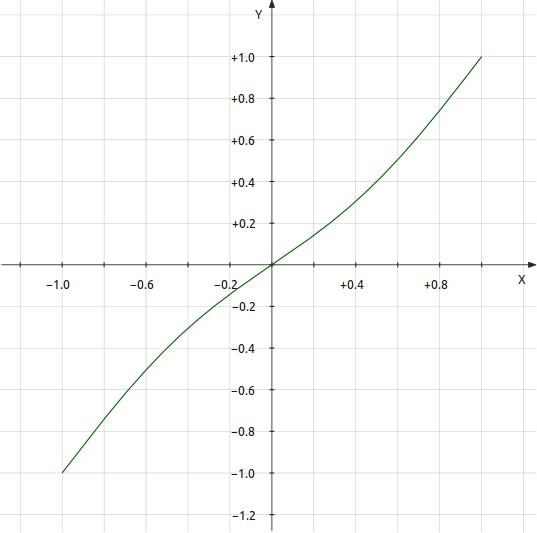
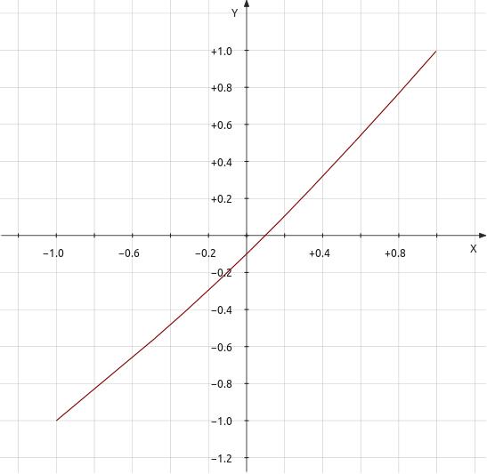
Figure 2: Transfer Curve 2 — y = x - k·sin(1.0π·x) |
|||||||||||||||||||||||||||||||||
 |
|||||||||||||||||||||||||||||||||
k = 0.000128746 Total distortion = 0.0001002025 0.01002025% -79.9824dB Breakdown by harmonic
|
|||||||||||||||||||||||||||||||||
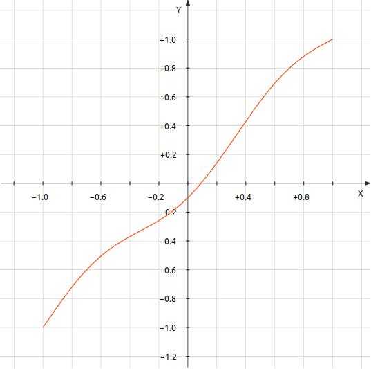
Figure 3: Transfer Curve 3 — y = x - k·cos(1.5π·x) |
|||||||||||||||||||||||||||||||||
 |
|||||||||||||||||||||||||||||||||
k = 7.9155e-005 Total distortion = 0.0001001989 0.01001989% -79.9827dB Breakdown by harmonic
|
|||||||||||||||||||||||||||||||||
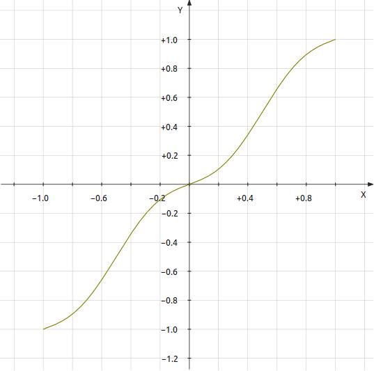
Figure 4: Transfer Curve 4 — y = x - k·sin(2.0π·x) |
|||||||||||||||||||||||||||||||||
 |
|||||||||||||||||||||||||||||||||
k = 8.4877e-005 Total distortion = 0.0001004889 0.01004889% -79.9576dB Breakdown by harmonic
|
|||||||||||||||||||||||||||||||||
Figure 5: Transfer Curve 5 — y = x - k·cos(2.5π·x) |
|||||||||||||||||||||||||||||||||
 |
|||||||||||||||||||||||||||||||||
k = 6.00815e-005 Total distortion = 0.0001006654 0.01006654% -79.9424dB Breakdown by harmonic
|
You should not read too much into the fact the the harmonic results are entirely even or odd. This is a function of the perfect symmetry of the trigonometric error functions used. However there is a trend here. The more bends in the transfer function, the higher the order of the highest harmonics that result.
Topology Considerations
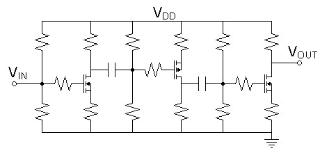
Care must be taken if successive stages of a system are not to create multiple bends in the transfer curve. It is commonly thought that bending the transfer function in an opposite directions alternatively will reduce distortion. And it may. However the nature of most transfer functions prevents distortion cancellation. Instead the flatter curve will have more bends. This is because the transfer curves of known amplifying devices have a slope that increases with magnitude, resulting in the greatest bend near cutoff. Alternate bends under varying gain and bias contexts will create random bends to a less musical end. A common topology creating an opportunity for multiple bends is one where the same polarity of device is used in successsive inverting stages (See figure 6 below). Vacuum tube circuits force this type of topology in some cases because tubes have only n-type transfer curves. Perhaps this is why SET fans scorn multiple amplifiying stages in their signal paths, sometimes only putting a passive volume control in front of their single-stage amp. Transistors have an advantage here because n-type and p-type devices are available enabling an alternating topology to match the bends in the transfer curves in the same direction relative to the signal (See figure 7 below).Figure 6: cascaded n-channel topology can create as many bends in the transfer curve as inverting stages. |
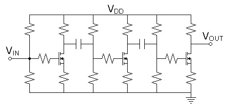 |
Figure 7: Alternating topology bends the transfer curve in the same direction relative to the signal in each device. |
 |
Dominant Bend Masking
Perhaps one might think to overcome transfer function anomalies by having one characteristic or bend in a transfer function dominate the others. Will the dominant bend solely determine the distortion outcome? First I added the error term of transfer curve 5 reduced by 10 to transfer curve 1 then determined this an improper model. The proper model below nests the transfer functions instead, a more proper representation. The result is somewhat inconclusive. Relative to multibend transfer curve, the second harmonic is raised, the fourth lowered, odds are added at low levels, the remainder lower. The result appears mostly additive with some subtractions due to phase. It appears the intended masking that results would be less than ideal. This might infer that using a euphonic stage to mask the distortion of a less than euphonic signal chain would require that chain to already have inaudible distortion.| Figure 8:
Transfer
Curve 6 —
y = x -
0.1k·cos(2.5π·x) - k·cos(0.5π·(x -
0.1k·cos(2.5π·x))) |
||||||||||||||||||||||||||||||||||||||||||||||||||||||||||||||||||||||||||||||||
 |
||||||||||||||||||||||||||||||||||||||||||||||||||||||||||||||||||||||||||||||||
| k = 0.000164986 Total distortion = 0.0001002453 0.01002453% -79.9787dB Breakdown by harmonic
|
Final Thoughts
Investigating the use of distortion cancellation in some topologies may add additional benefit to this pursuit. Other than a matched current mirror, I cannot immediately think of any circuit for which this would be an easy task. The expensive OPA627 operational amplifier derived its reputation for low distortion and quality sound from a proprietary distortion cancelling circuit.|
|
Document History
January 1, 2011 Created.
January 1, 2011 Made minor grammatical corrections.
January 6, 2011 Added investigation into distortion masking and
made an immediate model correction to same.