Home  │ Audio Home Page

Copyright © 2017 by Wayne Stegall
Updated July 14, 2017.  See Document History at end for details.

State Variable Tone Control

Introduction

Tone controls are often spoken of as harming audio sound.  Often capacitors are said to blame.  Here I propose that a state-variable tone control would diminish or eliminate capacitor distortion although replacing it with op amp distortion instead.

Preliminary Evaluation

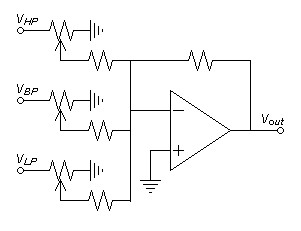
As an intuitive first try it seems that an integrator, a simple inverting stage, and a differentiators in the inner loop of an overall inverting stage with equal global feedback from each would create the desired function.  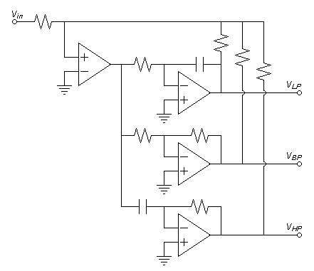The global feedback loop would force the sum of the three to be flat gain and as result the integrator output would become lowpass (bass), the inverting stage output would become bandpass (midrange), and the differentiator output would become highpass (treble).  This circuit is shown in figure 1 and its SPICE model in figure 2.

(1)

Hsum-inner-loop(s) =

s ωhp

+

1

+

ωlp s

Figure 1:  First schematic.

Figure 2:  First SPICE model.

* xover 300 and 5kHz v1 vin 0 dc 0 ac 1 sin 1.41421 0 rin vin 0 47k emain emo 0 emvp 0 100k r1 vin emvp 10k rfi emvp eio 10k rfu emvp euo 10k rfd emvp edo 10k eint eio 0 0 eivn 100k ri1 emo eivn 10k ci1 eivn eio 53n euni euo 0 0 euvn 100k ru1 emo euvn 10k ru2 euvn euo 10k ediff edo 0 0 edvn 100k cd1 emo edvn 6.77n rd1 edvn edo 4.7k .end .control ac dec 30 2 200k plot db(eio) db(euo) db(edo) plot db(eio+euo+edo) .endc

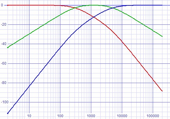
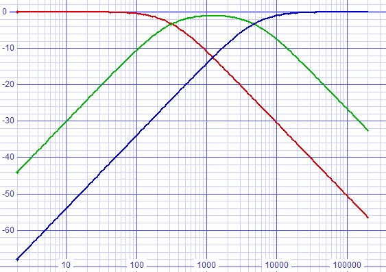
The bode plot from the SPICE emulation shows an anomaly.  Where the lowpass section was desired to have a single pole at ω_lp, it instead has another pole at ω_hp after which it rolls off with second order slope.  The highpass section is affected in a similar way.  Each section is divided by the summed response to get the flat summed result giving two poles to each section.

Figure 3:  Bode plot shows two poles each for lowpass and highpass functions.:

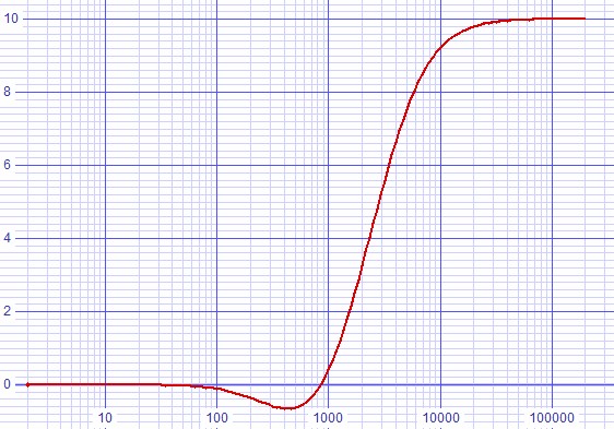
This seems acceptable until one of the sections is adjusted then the extra phase shift creates a response anomaly.  Figure 4 below shows the anomaly in the summed response with treble boost.

Figure 4:  Treble boost reveals two pole anomaly.

Add Compensating Zeros

It seems now that zeros have to be added to the integrator and differentiator to eliminate second-order response from the lowpass and highpass sections.  Now since intuition has failed, proceed by fully calculating all parameters.

Derive equations

First calculate the summed response which inverted becomes the midrange curve.  Begin with separate poles and zeros.

(2)

Hsum′(s) =

(s + ωlp)(s + ωhp) s

Multiply them together.

(3)

Hsum′(s) =

s2 + s(ωlp + ωhp) + ωlpωhp s

Divide numerator by denominator to distinguish integrator, flat, and differentiator functions.

(4)

Hsum′(s) =

s + (ωlp + ωhp) +

ωlpωhp s

Divide by ω_hp to attain normal scale.

(5)

Hsum(s) =

H′(s) ωhp

=

s ωhp

+

ωlp + ωhp ωhp

+

ωlp s

Show scaled pole/zero form for completeness.

(6)

Hsum(s) =

(s + ωlp)(s + ωhp) sωhp

Add zero at ω_hp to integrator.

(7)

Hint+zero(s) =

ωlp s

+

ωlp ωhp

=

(s + ωhp)ωlp sωhp

Divide integrator response by summed response to reveal lowpass function.

(8)

Hlp(s) =

(s + ωhp)ωlp sωhp (s + ωlp)(s + ωhp) sωhp

=

ωlp s + ωlp

Add zero at ω_lp to differetiator.

(9)

Hdiff+zero(s) =

s ωhp

+

ωlp ωhp

=

s + ωlp ωhp

Divide differetiator response by summed response to reveal highpass function.

(10)

Hhp(s) =

s + ωlp ωhp (s + ωlp)(s + ωhp) sωhp

=

s s + ωhp

Obtain function of flat-response section by subtracting the integrator and differentiator functions with zeros from the summed response.

(11)	Hflat(s) = Hsum(s) – Hint+zero(s) – Hint+zero(s)

(12)

Hflat(s) =

s ωhp

+

ωlp + ωhp ωhp

+

ωlp s

–

ωlp s

+

ωlp ωhp

–

s ωhp

+

ωlp ωhp

(13)

Hflat(s) = 1 –

ωlp ωhp

Divide flat-response section response by summed response to reveal bandpass function.

(14)

Hbp(s) =

1 –  ωlp ωhp (s + ωlp)(s + ωhp) sωhp

=

s(ωhp – ωlp) (s + ωlp)(s + ωhp)

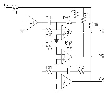
Now these calculations define the new circuit of figure 5 below.

Figure 5:  Second circuit adds zeros to integrator and differentiator sections.

Calculate circuit values.

Choose f_lp = 300Hz and f_hp = 5kHz.  Set primary resistances to 10kΩ.

(15)

Ci1 =

1 2πflpRi1

=

1 2π × 300Hz × 10kΩ

= 53.0516nF

(16)

Ri2 = Ri1 ×

flp fhp

= 10kΩ ×

300Hz 5kHz

= 600Ω

(17)

Cd1 =

1 2πfhpRd2

=

1 2π × 5kHz × 10kΩ

= 3.1831nF

(18)

Rd1 = Rd2 ×

fhp flp

= 10kΩ ×

5kHz 300Hz

= 166.667kΩ

(19)

Ru2 = Ru1

1 –

flp fhp

= 10kΩ

1 –

300Hz 5kHz

= 9.4kΩ

Run SPICE simulation

Figure 6:  Second SPICE deck using calculated values.

* xover 300 and 5kHz v1 vin 0 dc 0 ac 1 sin 1.41421 0 rin vin 0 47k emain emo 0 emvp 0 100k r1 vin emvp 10k rfi emvp eio 10k rfu emvp euo 10k rfd emvp edo 10k eint eio 0 0 eivn 100k ri1 emo eivn 10k ci1 eivn ri2ci1 53.0516n ri2 ri2ci1 eio 600 euni euo 0 0 euvn 100k ru1 emo euvn 10k ru2 euvn euo 9.4k ediff edo 0 0 edvn 100k cd1 emo edvn 3.183n rd1 emo edvn 166.667k rd2 edvn edo 10k .end .control ac dec 30 2 200k plot db(eio) db(euo) db(edo) plot db(eio+euo+edo) .endc

Figure 7:  Response now lacks the unwanted extra zeros.

Complete circuit

Now only a summer like that of figure 8 below need be attached to the output to adjust bass, midrange, and treble.

Figure 8:  Inverting Summer

Stability Design

If all of the op amps in the state variable circuit have the same bandwidth, the circuit is expected to oscillate.  A Texas Instruments paper says that if two op amps are in the same feedback loop, stability is possible if their bandwidths differ by a ratio of 5.¹  Even then experimentation is required.  There is much reason to believe that the wider bandwidth amps should be in the inner feedback loop functions for the following reasons:

• Wide bandwidth op amps prefer the shorted feedback paths.
• The inner loop amps with their feedback are more likely to reduce phase shift by the application of the inner feedback loops by the time the narrower bandwidth amps run out of gain.

If the choice of op amps does not produce stability, the ultrasonic gain of the differentiator may have to limited or returned to unity before the unity gain frequency of the outer loop amp is reached.

¹Ron Mancini, "Analyzing feedback loops containing secondary amplifiers," 2005, Texas Instruments, ti.com, link.

Document History
July 14, 2017  Created.
July 14, 2017  Corrected some grammar and omissions.
July 14, 2017  Added footnote validating reference referred in Stabiility Design..