Home  │ Audio Home Page

Copyright © 2014 by Wayne Stegall
Updated August 18, 2014.  See Document History at end for details.

Perspective

Introduction

Everyone has noticed the difference in the sizzle of lightning that strikes close by as compared to the low bass rumble of that from afar off.  Likewise, there is a perceived difference in frequency response of musical performances that conveys distance.  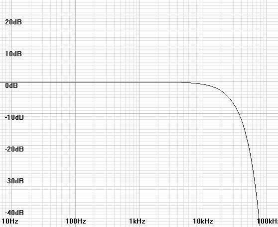The atmosphere obviously filters high frequencies in a manner related to the distance of transmission which the hearer then perceives as perspective indicating distance.  I submit that intervening air acts as lowpass filter in the form of distributed mass, compliance, and damping.  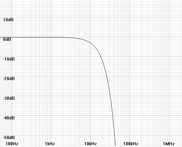Because this filter is effectively an infinite number of consecutive infinitesimal filters the response should then be an analog Gaussian filter of some cutoff frequency determined by distance.  This type of filter droops in the transition band like a Bessel or first-order lowpass filter and then falls off with increasing steepness in the stopband.

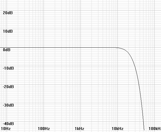
Figure 1:  Lowpass Gaussian (f0 = 10kHz)

Relating Frequency

Because Gaussians are usually specified for statistics, it becomes useful to respecify them by frequency response.

First write equation with unknown constant.

(1)

H(f) = e

–kf2

Then specify that same equation down -3dB at cutoff frequency f₀.

(2)

e

–kf02

=

1          2

Then solve for constant.

(3)

ln

e

–kf02

=  ln

1          2

(4)

–kf02 = –ln

2

(5)

k =

ln          2 f02

Relating Distance

Adding increments of distance is equivalent to joining consecutive filters of unit distance.  Consider first that filter magnitudes multiply.

(6)

H(f) = e

–k1f2

× e

–k2f2

× e

–k3f2

... × e

–knf2

Reducing the equation results in a useful result.

(7)

H(f) = e

-(k1+k2+k3 ... +kn)f2

Because the constants k₁ through k_n add in the exponent, that indicates that the distance is related in that way there.  Therefore if we set k_Dd = k₁+k₂+k₃ ... +k_n where d is distance and k_D is a new constant then:

(8)

H(f) = e

–kDdf2

If in addition we set:

(9)

kDd = k =

ln          2 f02

then frequency can be related to distance.

(10)

f02 =

ln          2 kDd

(11)

f0 =

ln          2 kDd spacessssssss

Ideal Equalization

Because the atmosphere is acting effectively as a mechanical Gaussian filter, perspective can be lengthened by adding an additional electronic Gaussian filter.  Likewise perspective can be shortened by adding an inverse Gaussian filter which is effectively like removing a section of the mechanical Gaussian so modified.

Lowering f₀ (or adding distance)

First quantify the addition of distance.

(12)

dnew = dold + dfilter

Then derive a relation to frequency from equations 10 and 12.

(13)

1 fnew2

=

1 fold2

+

1 ffilter2

Then a final form can be derived.

(14)

fnew =

1 1 fold2 + 1 ffilter2 spacesssssssssss

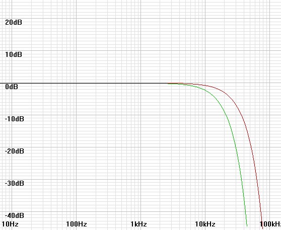
Example:  Calculate filter frequency to lower cutoff frequency from 20kHz to 10kHz.

Solution:
Rearrange equation 13 to obtain a filter cutoff frequency and solve.

(15)

ffilter =

1 1 fnew2 – 1 fold2 spacesssssssssss

=

1 1 10kHz2 – 1 20kHz2 spacessssssssssssssss

= 11.547kHz

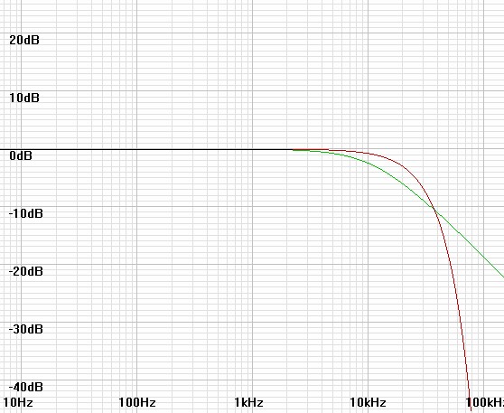
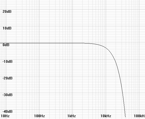
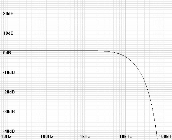
Figure 2:  Response of 20kHz cutoff perspective in red, that of applied filter of 11.547kHz cutoff in green.	Figure 3:  Combined response produces more distant perspective with 10kHz cutoff.

Raising f₀ (or subtracting distance)

First quantify the subtraction of distance.

(16)

dnew = dold – dfilter

Then derive a relation to frequency from equations 10 and 16.

(17)

1 fnew2

=

1 fold2

–

1 ffilter2

Then a final form can be derived.

(18)

fnew =

1 1 fold2 – 1 ffilter2 spacesssssssssss

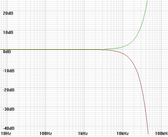
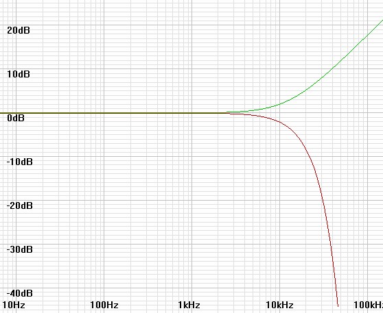
Example:  Calculate the filter frequency to raise the cutoff frequency from 12kHz to 20kHz

(19)

ffilter =

1 1 fold2 – 1 fnew2 spacesssssssssss

=

1 1 12kHz2 – 1 20kHz2 spacessssssssssssssss

= 15kHz

Figure 4:  Response of 12kHz-cutoff perspective in red, that of applied filter of 15kHz 3dB boost in green.	Figure 5:  Combined response produces closer perspective with 20kHz cutoff.

Practical Equalization

The Gaussian filters depicted to change the perspective above are only realizable as digital filters.  Because many would rather equalize using analog filters, I here explore the outcome of using first-order poles or zeros for equalization.

Lowering f₀ (or adding distance)

Because a first-order lowpass filter has similar droop in the transition band to that of a Gaussian, it is reasonable to think that a more distant perspective could be created using it in place of the ideal Gaussian filter.  In figures 6 and 7 below, I add a first-order filter of the same 11.547kHz cutoff frequency as the Gaussian and get plausible results.

Figure 6:  Response of 20kHz cutoff perspective in red, that of applied filter of 11.547kHz pole in green.	Figure 7:  Combined response produces more distant perspective with 10kHz cutoff, nearly as well as with adding the Gaussian filter above.

Raising f₀ (or subtracting distance)

When I added a filter of zero at the 15kHz calculated for an inverse Gaussian, the response at 20kHz was below the target of -3dB.  A zero at 12kHz produced a result with a small amount of ripple.  The third trial of a 13kHz zero produced the desired results.

Figure 8:  Response of 12kHz-cutoff perspective in red, that of applied filter of 13kHz zero in green.	Figure 9:  Combined response produces closer perspective with 20kHz cutoff.  However the transition band has less droop than the Gaussian result.

Limitations

Because the Gaussian response falls off so fast in the stopband, it seems that lengthening the perspective is a much easier task than shortening it.  Even shortening the perspective with the ideal inverse Gaussian is very limited if practical gain limits such as 20dB are imposed.  In that case the cutoff frequency can only be raised by a factor of 2.5 or so by inspection of figure 1 and less with a first-order analog zero.

Also because this acoustic effect varies greatly with atmospheric pressure, temperature, and humidity, it may be difficult to pin down exact Gaussian cutoff frequencies for real listening conditions.¹

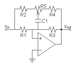
A Circuit

As for choice of analog equalizer, just a normal treble control with high pole/zero frequencies is recommended.  A control such as in figure 10 will have complimentary poles and zeros that cancel at the flat setting.  Then when adjusted, the zero drops in frequency and the pole rises when adjusted for boost and likewise the pole drops and the zero rises when adjusted for cut.  If the flat pole/zero frequency is set above 20kHz by enough that a clean pole or zero is brought into band on adjustment, then the desired equalization adjustment is facilitated.

Figure 10:  A high frequency treble adjustment

Parts List R1, R3 6kΩ R2, R4 1kΩ R5 10kΩ potentiometer C1 2.7nF

Note:  You may want to experiment with different values for effect on range of adjustment.

¹International Standard ISO 9613-1 "Acoustics – Attenuation of sound during propagation outdoors," 1993-06-01.  This document did not deal directly with the desired topic of Gaussian frequency response but rather with tabulating attenuation constants for distance for multiple variables of frequency, temperature, pressure, and humidity in other terms.

Document History
August 16, 2014  Created.
August 18, 2014  Corrected some misspellings and grammar, improved some wording, and completed footnote.