 |
| Home │ Audio
Home Page |
Copyright © 2012 by Wayne Stegall
Updated March 15, 2012. See Document History at end for
details.
One-Bend Amplifier
Part
2: Improving important details of a current-feedback amplifier
Introduction
I last said in the previous article that the one-bend amplifier was likely unfinished. When I did a slew rate analysis, I found it to be 3V/µs. Consider the following slew rate calculations:| (1) | vpk = |
2PR
|
= |
2 × 30W × 8Ω | = 21.91V |
| (2) |
minimum slew rate = 2πfvpk = 2π × 20kHz × 21.91V = 2.753V/µs |
In this case 3V/µs was inadequate for a this minimum calculated slew rate of 2.753V/µs. As a result the Fourier results for 20kHz at full power were very bad for the original one-bend circuit.
SPICE Model of Power Supply (for all circuits).
Improving Slew Rate
I deemed two improvements were necessary to remedy the problem with
slew rate. Slew rate was worst on pull than push. To
improve the pull, I added a current source in parallel with the
resistor loading stage 1. Then because slew is a matter of
limited current driving capacitance, I increased the bias for stages 1
and 2: stage 1 from 1mA to 10mA, and stage 2 from 45mA to
119mA. The 119mA bias was to dissipate 4W per M1 and M2
based on full utilization of common 5W TO220 heat sinks. In the
first stage, I paired the JFETs and specified the higher current rated
C version to give current margin over the new 10mA bias. To
simplify setup, I changed the adjustable M2 MOSFET current source to
one fixed by the stable VBE voltage of an NPN
transistor. The
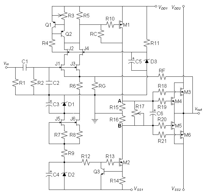
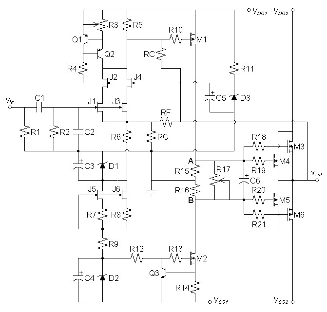
result is the following circuit.| Figure
1:
Current-feedback
amplifier
corrected
for
higher
slew
rate |
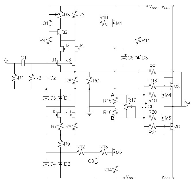 |
| SPICE Model |
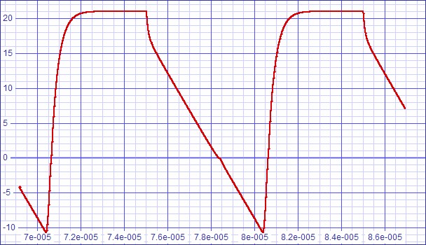
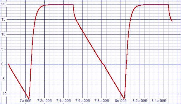
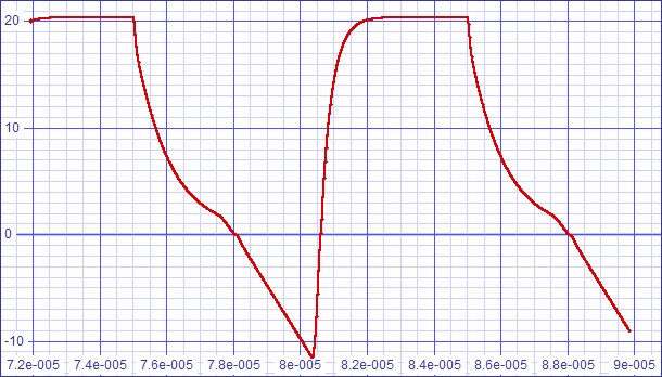
| Figure 2: Slew rate
analysis shows dv/dt of 5.2V/µs good for 37.77kHz power bandwidth |
 |
Fourier analysis at 1kHz for vout:
No. Harmonics: 16, THD: 0.0012549 %, Gridsize: 200, Interpolation Degree: 3
| Harmonic | Frequency | Magnitude | |
Norm.Mag | |
Percent | |
Decibels |
| -------- | --------- | --------- | --------- | --------- | --------- | |||
| 1 | 1000 | 21.8095 | 1 | 100 | 0 | |||
| 2 | 2000 | 0.000258371 | 1.18467E-05 | 0.00118467 | -98.5281 | |||
| 3 | 3000 | 0.000058014 | 2.66003E-06 | 0.000266003 | -111.502 | |||
| 4 | 4000 | 0.000039892 | 1.82911E-06 | 0.000182911 | -114.755 | |||
| 5 | 5000 | 3.77342E-05 | 1.73017E-06 | 0.000173017 | -115.238 | |||
| 6 | 6000 | 1.46938E-05 | 6.73733E-07 | 6.73733E-05 | -123.430 | |||
| 7 | 7000 | 3.41571E-05 | 1.56615E-06 | 0.000156615 | -116.103 | |||
| 8 | 8000 | 2.11585E-06 | 9.70147E-08 | 9.70147E-06 | -140.263 | |||
| 9 | 9000 | 9.57353E-06 | 4.38961E-07 | 4.38961E-05 | -127.151 | |||
| 10 | 10000 | 8.64029E-06 | 3.9617E-07 | 0.000039617 | -128.042 | |||
| 11 | 11000 | 6.54572E-06 | 3.00131E-07 | 3.00131E-05 | -130.454 | |||
| 12 | 12000 | 7.97776E-06 | 3.65792E-07 | 3.65792E-05 | -128.735 | |||
| 13 | 13000 | 9.20586E-06 | 4.22103E-07 | 4.22103E-05 | -127.492 | |||
| 14 | 14000 | 2.35572E-06 | 1.08013E-07 | 1.08013E-05 | -139.330 | |||
| 15 | 15000 | 4.34586E-06 | 1.99264E-07 | 1.99264E-05 | -134.011 |
Although distortion is not as low as at 1kHz, Fourier analysis at 20kHz proves slew rate improvement largely successful.
No. Harmonics: 16, THD: 0.0573418 %, Gridsize: 200, Interpolation Degree: 3
| Harmonic | Frequency | Magnitude | |
Norm.Mag | |
Percent | |
Decibels |
|
|
|
|
|
|
|
|||
| 1 | 20000 | 21.7961 | 1 | 100 | 0 | |||
| 2 | 40000 | 0.0056118 | 0.000257469 | 0.0257469 | -71.7855 | |||
| 3 | 60000 | 0.00956154 | 0.000438682 | 0.0438682 | -67.157 | |||
| 4 | 80000 | 0.000835605 | 3.83374E-05 | 0.00383374 | -88.3275 | |||
| 5 | 100000 | 0.00464674 | 0.000213192 | 0.0213192 | -73.4246 | |||
| 6 | 120000 | 0.00051708 | 2.37235E-05 | 0.00237235 | -92.4964 | |||
| 7 | 140000 | 0.00266117 | 0.000122094 | 0.0122094 | -78.2661 | |||
| 8 | 160000 | 0.000421559 | 1.93411E-05 | 0.00193411 | -94.2704 | |||
| 9 | 180000 | 0.00154427 | 7.08509E-05 | 0.00708509 | -82.9931 | |||
| 10 | 200000 | 0.000349586 | 1.60389E-05 | 0.00160389 | -95.8965 | |||
| 11 | 220000 | 0.000830694 | 3.81121E-05 | 0.00381121 | -88.3787 | |||
| 12 | 240000 | 0.000293413 | 1.34617E-05 | 0.00134617 | -97.418 | |||
| 13 | 260000 | 0.000357373 | 1.63962E-05 | 0.00163962 | -95.7051 | |||
| 14 | 280000 | 0.000247156 | 1.13395E-05 | 0.00113395 | -98.9081 | |||
| 15 | 300000 | 4.02591E-05 | 1.84708E-06 | 0.000184708 | -114.67 |
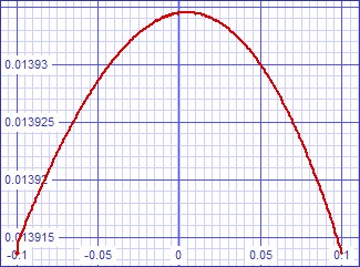
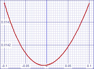
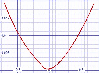
| Figure
3: Small signal transfer error curve |
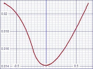
Figure
4: Large signal transfer error curve |
 |
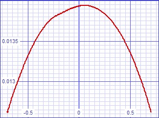 |
| The slight kink is
attributable to SPICE convergence difficulties, actual curve is likely
as smooth as the small signal one on the left. |
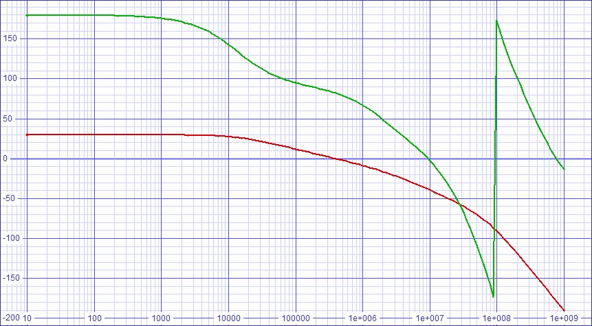
| Figure
5:
Stability
analysis
for
slew
rate
improved
circuit. |
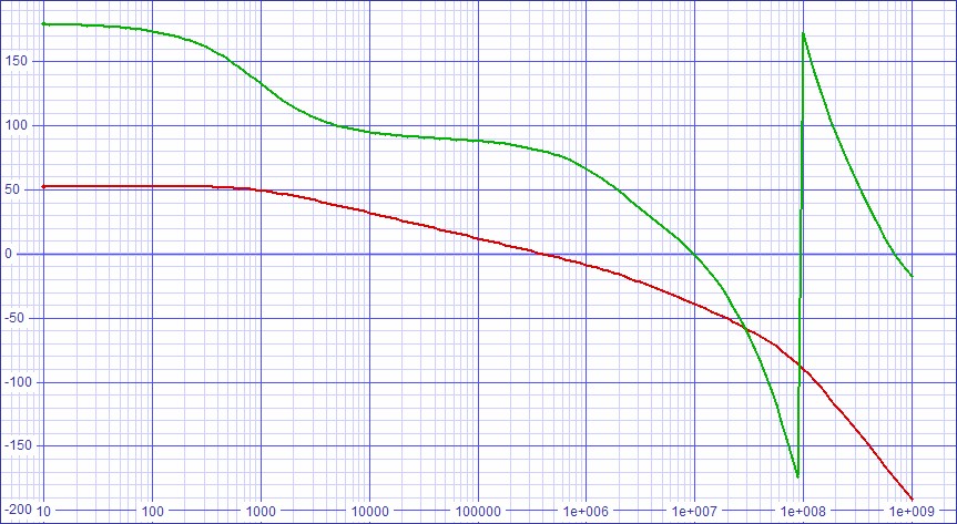 |
The stability analysis show and outstanding 80 degrees of phase margin. However, although the 1kHz dominant pole is better than one at 10Hz, one ≥ 10kHz is desired.
Raising the Dominant Pole Frequency
By plotting the stability analysis more specifically, I determined that
the 1kHz dominant pole was determined largely by the interaction
between the load resistance of stage one and the Miller capacitance
seen at the input of M1. Therefore, I sought to lower the Miller
capacitance by reducing the gain of the second stage. Using a
source resistor on M1 to lower the gain would also limit the positive
voltage swing. As a result I decided to add the local feedback
between the drain and gate resistor of M1. This addition changes
the circuit to that of figure 6
below. To avoid the tedium of complex calculations, I tried a
100kΩ for the new component RC and got excellent results.| Figure 6: Current-feedback amplifier improved for higher dominant pole. |
 |
| SPICE Model |
| Figure 7: Slew rate still
holds at dv/dt = 5.2V/µs |
 |
Fourier analysis at 1kHz for vout:
No. Harmonics: 16, THD: 0.00624645 %, Gridsize: 200, Interpolation Degree: 3
| Harmonic | Frequency | Magnitude | |
Norm.Mag | |
Percent | |
Decibels |
|
|
|
|
|
|
|
|||
| 1 | 1000 | 20.6212 | 1 | 100 | 0 | |||
| 2 | 2000 | 0.00121863 | 5.90959E-05 | 0.00590959 | -84.5689 | |||
| 3 | 3000 | 0.000318355 | 1.54382E-05 | 0.00154382 | -96.2281 | |||
| 4 | 4000 | 0.000184075 | 8.92648E-06 | 0.000892648 | -100.986 | |||
| 5 | 5000 | 0.000167846 | 8.13948E-06 | 0.000813948 | -101.788 | |||
| 6 | 6000 | 4.15484E-05 | 2.01483E-06 | 0.000201483 | -113.915 | |||
| 7 | 7000 | 8.79902E-05 | 4.26697E-06 | 0.000426697 | -107.398 | |||
| 8 | 8000 | 1.05453E-05 | 5.11378E-07 | 5.11378E-05 | -125.825 | |||
| 9 | 9000 | 9.64684E-06 | 4.67811E-07 | 4.67811E-05 | -126.599 | |||
| 10 | 10000 | 2.04371E-05 | 9.91068E-07 | 9.91068E-05 | -120.078 | |||
| 11 | 11000 | 1.75095E-05 | 8.49097E-07 | 8.49097E-05 | -121.421 | |||
| 12 | 12000 | 0.000011695 | 5.67135E-07 | 5.67135E-05 | -124.926 | |||
| 13 | 13000 | 1.34944E-05 | 6.54395E-07 | 6.54395E-05 | -123.683 | |||
| 14 | 14000 | 1.77303E-06 | 8.59805E-08 | 8.59805E-06 | -141.312 | |||
| 15 | 15000 | 2.52197E-06 | 1.22299E-07 | 1.22299E-05 | -138.252 |
Fourier analysis at 20kHz for vout:
No. Harmonics: 16, THD: 0.0506489 %, Gridsize: 200, Interpolation Degree: 3
| Harmonic | Frequency | Magnitude | Norm.Mag | Percent | Decibels |
|
|
|
|
|
|
|
| 1 | 20000 | 20.6027 | 1 | 100 | 0 |
| 2 | 40000 | 0.00374705 | 0.000181872 | 0.0181872 | -74.8047 |
| 3 | 60000 | 0.00848886 | 0.000412027 | 0.0412027 | -67.7015 |
| 4 | 80000 | 0.000622974 | 3.02376E-05 | 0.00302376 | -90.3891 |
| 5 | 100000 | 0.00394035 | 0.000191254 | 0.0191254 | -74.3678 |
| 6 | 120000 | 0.000462974 | 2.24716E-05 | 0.00224716 | -92.9673 |
| 7 | 140000 | 0.00215136 | 0.000104422 | 0.0104422 | -79.6242 |
| 8 | 160000 | 0.000376485 | 1.82736E-05 | 0.00182736 | -94.7635 |
| 9 | 180000 | 0.00116204 | 5.64023E-05 | 0.00564023 | -84.9741 |
| 10 | 200000 | 0.000309166 | 1.50061E-05 | 0.00150061 | -96.4746 |
| 11 | 220000 | 0.000545727 | 2.64882E-05 | 0.00264882 | -91.539 |
| 12 | 240000 | 0.000256768 | 1.24629E-05 | 0.00124629 | -98.0876 |
| 13 | 260000 | 0.000147549 | 7.16162E-06 | 0.000716162 | -102.9 |
| 14 | 280000 | 0.000215353 | 1.04527E-05 | 0.00104527 | -99.6154 |
| 15 | 300000 | 0.000109782 | 5.32853E-06 | 0.000532853 | -105.468 |
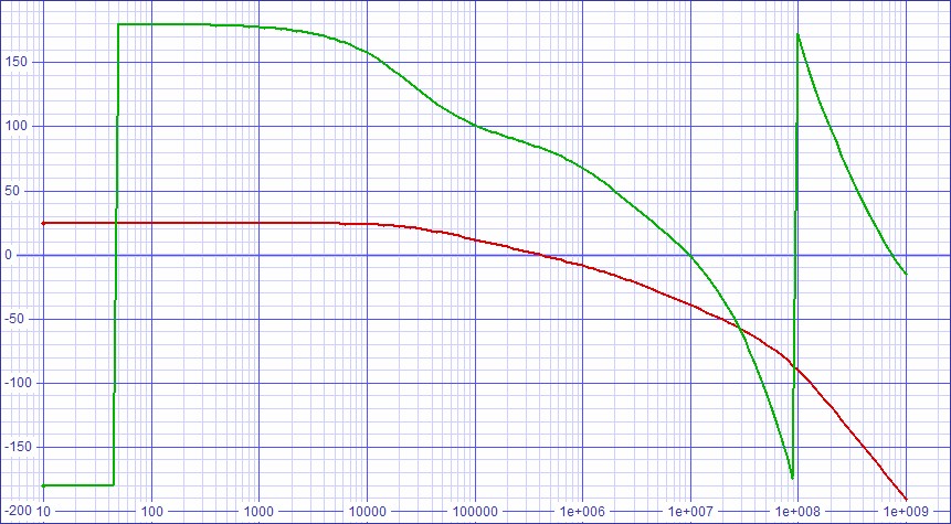
| Figure
8:
Stability
analysis
shows
a
dominant
pole
of
about
23kHz |
 |
| Figure 9: Small signal transfer error curve | Figure 10: Large signal transfer error curve |
 |
 |
Can It Be Made to Meet all Specifications?
Having lost a one-bend curve to gain a desirable dominant pole, I had
to think of a change that would gain both for me without losing some
other quality.
After altering the previous circuit in every possible way without
avail, I decided to tap the local feedback off of the output instead of
the drain of M1. This is now actually a multiple feedback
configuration.| Figure 11: Current-feedback amplifier improved for higher dominant pole |
 |
| SPICE Model |
Since I chose RC for the desired dominant pole in the process of making the circuit change, I was most eager to see the transfer curves. They turned out well with R15 and R16 set at 1.8kΩ for somewhat low second stage gain. The open-loop stability analysis showed a dominant pole slightly above my 10kHz target with 82 degrees of phase margin. Last of all, I verified that slew rate was not lost in perfecting the other qualities.
| Figure 12: Small signal transfer error curve | Figure 13: Large signal transfer error curve |
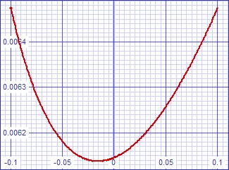 |
 |
| The
slight kink in the large signal curve is
attributable to SPICE convergence difficulties; the small signal one on
the left shows a nice smooth curve in the same range. |
Fourier analysis at 1kHz for vout:
No. Harmonics: 16, THD: 0.016281 %, Gridsize: 200, Interpolation Degree: 3
| Harmonic | Frequency | Magnitude | |
Norm.Mag | |
Percent | |
Decibels |
|
|
|
|
|
|
|
|||
| 1 | 1000 | 21.1525 | 1 | 100 | 0 | |||
| 2 | 2000 | 0.00343828 | 0.000162547 | 0.0162547 | -75.7804 | |||
| 3 | 3000 | 0.000172863 | 8.1722E-06 | 0.00081722 | -101.753 | |||
| 4 | 4000 | 5.42204E-05 | 2.5633E-06 | 0.00025633 | -111.824 | |||
| 5 | 5000 | 3.67777E-05 | 1.73869E-06 | 0.000173869 | -115.196 | |||
| 6 | 6000 | 3.36128E-05 | 1.58907E-06 | 0.000158907 | -115.977 | |||
| 7 | 7000 | 2.07878E-05 | 9.82755E-07 | 9.82755E-05 | -120.151 | |||
| 8 | 8000 | 1.78872E-05 | 8.4563E-07 | 0.000084563 | -121.456 | |||
| 9 | 9000 | 0.000032523 | 1.53754E-06 | 0.000153754 | -116.263 | |||
| 10 | 10000 | 8.33138E-06 | 3.93871E-07 | 3.93871E-05 | -128.093 | |||
| 11 | 11000 | 2.70611E-05 | 1.27933E-06 | 0.000127933 | -117.86 | |||
| 12 | 12000 | 6.4671E-06 | 3.05736E-07 | 3.05736E-05 | -130.293 | |||
| 13 | 13000 | 0.000015963 | 7.54663E-07 | 7.54663E-05 | -122.445 | |||
| 14 | 14000 | 8.20451E-06 | 3.87873E-07 | 3.87873E-05 | -128.226 | |||
| 15 | 15000 | 5.42339E-06 | 2.56394E-07 | 2.56394E-05 | -131.822 |
Fourier analysis at 20kHz for vout:
No. Harmonics: 16, THD: 0.066975 %, Gridsize: 200, Interpolation Degree: 3
| Harmonic | Frequency | Magnitude | |
Norm.Mag | |
Percent | |
Decibels |
|
|
|
|
|
|
|
|||
| 1 | 20000 | 21.1391 | 1 | 100 | 0 | |||
| 2 | 40000 | 0.00402414 | 0.000190365 | 0.0190365 | -74.4083 | |||
| 3 | 60000 | 0.0105682 | 0.000499935 | 0.0499935 | -66.0217 | |||
| 4 | 80000 | 0.000838083 | 3.96461E-05 | 0.00396461 | -88.036 | |||
| 5 | 100000 | 0.00607038 | 0.000287164 | 0.0287164 | -70.8374 | |||
| 6 | 120000 | 0.000507738 | 2.40189E-05 | 0.00240189 | -92.3889 | |||
| 7 | 140000 | 0.00413665 | 0.000195687 | 0.0195687 | -74.1688 | |||
| 8 | 160000 | 0.000384928 | 1.82093E-05 | 0.00182093 | -94.7941 | |||
| 9 | 180000 | 0.00296947 | 0.000140473 | 0.0140473 | -77.0481 | |||
| 10 | 200000 | 0.000319767 | 1.51268E-05 | 0.00151268 | -96.4051 | |||
| 11 | 220000 | 0.00215871 | 0.000102119 | 0.0102119 | -79.8179 | |||
| 12 | 240000 | 0.000289091 | 1.36756E-05 | 0.00136756 | -97.2811 | |||
| 13 | 260000 | 0.00157256 | 7.43912E-05 | 0.00743912 | -82.5696 | |||
| 14 | 280000 | 0.000265267 | 1.25486E-05 | 0.00125486 | -98.0281 | |||
| 15 | 300000 | 0.00113568 | 5.37244E-05 | 0.00537244 | -85.3966 |
| Figure 14: Open-loop
stability plot shows dominant pole > 10kHz and phase margin of 82
degrees. |
 |
| Figure 15: Slew rate drops slightly to 5.0V/µs |
 |
Last Thoughts
The one-bend ideas seems in the end only to increase the odds of a
one-bend result. Negative feedback appears to be able to alter
the transfer
curve in capricious ways that are very hard to pin down.
Therefore, no presumption can be inferred about a distortion outcome
with out attention to every detail.The slew rate, though now acceptable, is still short of what most would like and perhaps still leaves the design incomplete.
Links
Previous article: One-Bend Amplifier January 31, 2012. Part 1: Compare a current-feedback amplifier allowing a one-bend distortion characteristic to its voltage-feedback equivalent.|
|
Document History
March 14, 2012 Created.
March 15, 2012 Corrected some grammar and made some minor changes to wording.